Fine Tuning Faster RCNN ResNet50 FPN V2 using PyTorch

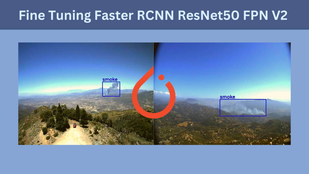
Faster RCNN models are two stage object detectors. Over the years, although slower compared to the latest models, they have proved to be some of the best models. In this blog post, we will be fine tuning the Faster RCNN ResNet50 FPN V2 model on a challenging dataset. We will use the PyTorch framework for this.

Faster RCNN object detection models are great at dealing with complex datasets and small objects. Although we will not be dealing with any small object detection in this post, we will use a challenging dataset for smoke detection.

As of now, PyTorch provides new and improved versions of Faster RCNN models, namely, Faster RCNN ResNet50 FPN V2. Fine tuning the Faster RCNN ResNet50 FPN V2 model should give superior results compared to its predecessor. We will also check this by comparing the detection results of both models.

We will cover the following points in this tutorial:

• As we will use a smoke detection dataset in this post, we will start by exploring that.
• Next, we will explore the code and directory structure for the project.
• For the coding part, we will go through some of the important code snippets.
• Then we will train the Faster RCNN ResNet50 FPN V2 model and also run inference using the trained model.
• Finally, we will compare the new ResNet50 FPN V2 model with the ResNet50 FPN model. This will give us a good idea of how much better the new Faster RCNN ResNet50 FPN V2 is.

The Smoke Detection Dataset

In this blog post, we will be using the Smoke Detection dataset from Kaggle for fine tuning the Faster RCNN ResNet50 FPN V2 model.

As the name suggests, the dataset contains images of smoke from hilltops or forests taken from an overview camera (probably a drone camera).

The entire dataset contains 737 images. The annotations are in the Pascal VOC (XML files) format. There is only one object class in the dataset, that is, smoke.

The following are a few images from the dataset with their annotations.

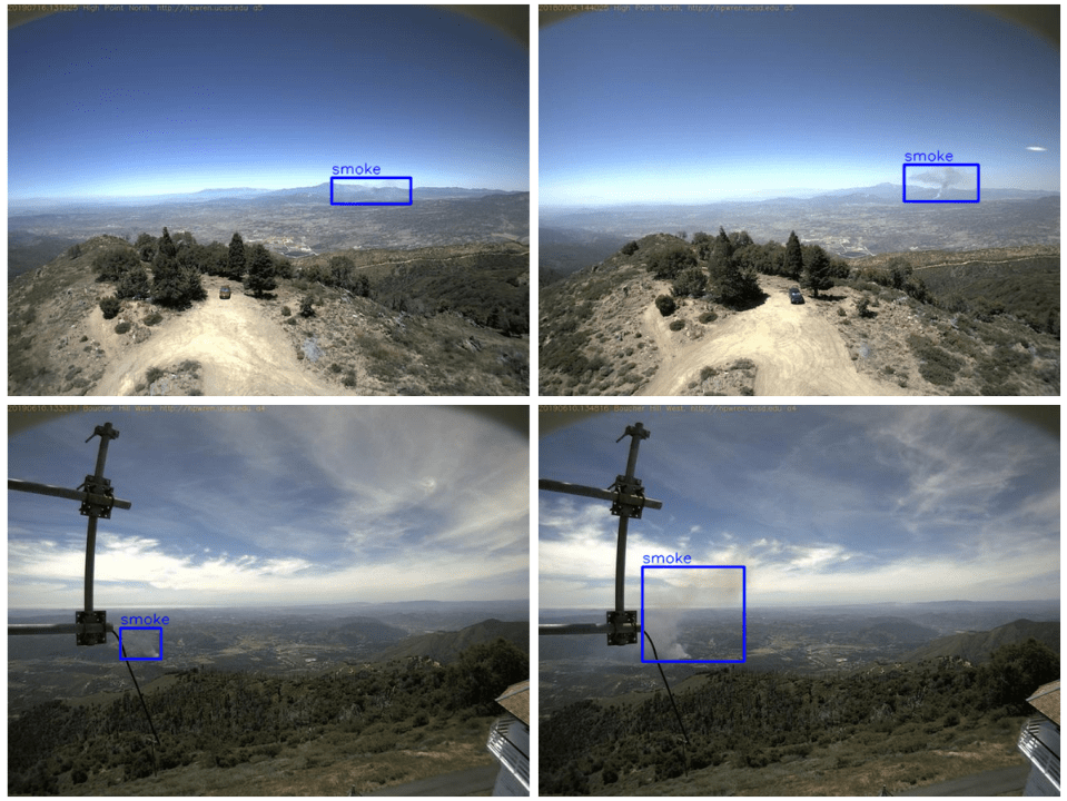
Our objective is to train an object detection model that can detect smoke emissions just as in the images in the dataset.

It may seem fairly simple in the beginning, but as we will see later, it is a slightly complicated problem. Getting accurate detections would mean avoiding ambiguity in cases of multiple closely spaced smoke emissions. Also, the amount of area a particular smoke emission is covering can be hard to figure out for a detection algorithm.

You may download the dataset now. Later in the post, we will split the dataset into a training and validation set.

Directory Structure

The following is the directory structure for the project.

.
├── data
│   ├── annotations # From the original dataset.
│   ├── images # From the original dataset.
│   ├── inference_data # Contains videos/images for inference.
│   ├── train_images # Manual-split training images.
│   ├── train_xmls # Manual-split training XML files.
│   ├── valid_images # Manual-split validation images.
│   ├── valid_xmls # Manual-split validation XML files.
│   └── smoke-pascal-voc.zip
├── data_configs
│   └── smoke.yaml
├── models
│   ├── create_fasterrcnn_model.py
│   ├── fasterrcnn_resnet50_fpn.py
│   ├── fasterrcnn_resnet50_fpn_v2.py
│   └── __init__.py
├── outputs
│   ├── inference
│   └── training
├── torch_utils
│   ├── coco_eval.py
│   ├── coco_utils.py
│   ├── engine.py
│   ├── __init__.py
│   └── utils.py
├── utils
│   ├── annotations.py
│   ├── general.py
│   ├── __init__.py
│   ├── logging.py
│   └── transforms.py
├── datasets.py
├── inference.py
├── inference_video.py
├── random_split.py
├── requirements.txt
└── train.py

• The data directory contains all the files (images and annotations) related to the dataset. The annotations and images subdirectories are the ones that we get after extracting the zip file from the original dataset. We create training and validation splits for both, the images and annotations, which we can see in the above code block.
• The data_configs contains a YAML file with the dataset information to be used while training the model.
• In the models directory, we have three scripts. Two of them are for the two versions of the Faster RCNN model (V1 and V2). And the create_fasterrcnn_model.py is the one that calls the functions in the two model files that return the model object.
• The outputs directory will contain all the training and inference outputs.
• In the torch_utils directory, we have several scripts that drive the training. These include code for training and validation loops as well as code to calculate the COCO mAP metrics.
• The utils directory contains some custom utility code. These are for annotating images, saving training and validation plots, logging, and applying transformations.
• Directly inside the project directory, we have a few scripts as well. The datasets.py contains the code to prepare the training and validation data loaders. inference.py and inference_video.py are for running inference on images and videos respectively. The random_split.py script is for creating training and validation splits out of the original dataset. We will use this later to do the same. The train.py script is the executable script that will drive the training.

There are a lot of code files in the project. We will not go through all of them but only through a few important code snippets. By downloading the zip file for this project, you will get access to all the scripts with the directory structure. You just have to prepare the dataset.

PyTorch Version

To run the code in this blog post, you will need at least PyTorch 1.12.0.

Download Code

You can use the requirements.txt file to install all the requirements for this project. If you are on Linux (Kaggle and Google Colab environment as well), just execute the following command in the choice of your Anaconda/Python virtual environment.

pip install -r requirements.txt

This should install all the dependencies for the project.

Before moving further, if you are new to Faster RCNN models, or object detection, then don’t miss out on the other amazing posts on DebuggerCafe.

• How to Train Faster RCNN ResNet50 FPN V2 on Custom Dataset?
• Object Detection using PyTorch Faster RCNN ResNet50 FPN V2

The Faster RCNN ResNet50 FPN V2 Fine Tuning Code

The code that we use in this blog post is part of a much bigger project. It has been taken from the Faster RCNN Training Pipeline project on GitHub.

For brevity and to keep things simple, we only use the absolutely necessary parts. These include:

• Logging the training procedure from the terminal into a train.log file.
• Saving all the Mean Average Precision and loss plots.
• Saving the best model to disk that we will use for inference.
• Use mosaic augmentation along with more advanced augmentations.

A Small Heads Up About Mosaic Augmentation

Nowadays, using the proper data augmentation techniques is absolutely critical for the success of any object detection project.

Mosaic augmentation is one of the more advanced techniques. It cannot be used for all datasets. But wherever it can be used, it works really well.

For that reason, it is an essential part of the data augmentation techniques that we use in this code base along with some other augmentations.

For example, take a look at the following figure.

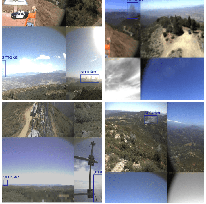
The above figure shows a few images from the training data loader pipeline. In mosaic augmentation, four images are stitched together with different crop ratios. Moreover, we can see the effect of some other augmentation as well. These include:

• MotionBlur
• Blur
• RandomBrightnessContrast
• RandomGamma
• RandomFog

All these augmentations have been applied using the Albumentations library.

Fine Tuning Faster RCNN ResNet50 FPN V2 on the Smoke Detection Dataset

Starting here, we will get into the coding part of the post now.

Preparing the Training and Validation Sets

The original dataset came with one folder for images and one folder for annotations. But we need to split the dataset into a training and validation set.

If you have downloaded the code for this post, you can just execute the random_split.py script to do so.

python random_split.py

This creates the corresponding training and validation splits for the images and XML files. We are using 17% of the dataset for validation and the rest for training.

In the previous post, we discussed the training process of Faster RCNN ResNet50 FPN V2. We also covered the code for constructing the model. If you want to learn about the model code, please go through the previous post.

Here, we will only discuss the dataset YAML file.

The Smoke Detection Dataset YAML File

The dataset YAML file resides inside the data_configs directory.

The following are the contents of smoke.yaml file.

# Images and labels direcotry should be relative to train.py
TRAIN_DIR_IMAGES: 'data/train_images'
TRAIN_DIR_LABELS: 'data/train_xmls'
VALID_DIR_IMAGES: 'data/valid_images'
VALID_DIR_LABELS: 'data/valid_xmls'

# Class names.
CLASSES: [
    '__background__',
    'smoke'
]

# Number of classes (object classes + 1 for background class in Faster RCNN).
NC: 2

# Whether to save the predictions of the validation set while training.
SAVE_VALID_PREDICTION_IMAGES: True

First, we define the paths to the training and validation images along with the paths to the XML files.

Then we define the classes. In this dataset, we have the smoke class only. The __background__ is an additional mandatory class that we need for training Faster RCNN models. So, the total number of classes, NC becomes 2.

Finally, we have the SAVE_VALID_PREDICTION_IMAGES set to True. This tells the training script that we want to save a few images from the validation set in the result directory along with their predictions. This makes it easier for us to evaluate the progress of the model qualitatively as well.

Training the Faster RCNN ResNet50 FPN V2 Model

Note: If you intend to train the model on your local system, please ensure that you do so on a GPU. The following training and inference experiments were conducted on a machine with 10 GB RTX 3080 GPU, 32 GB of RAM, and an Intel Core i7 10th generation CPU.

The train.py script contains the executable code that drives the entire training process.

To train the model, we just need to execute the following command in the terminal.

python train.py --model fasterrcnn_resnet50_fpn_v2 --epochs 25 --batch-size 4 --workers 4 --project-name smoke_detection_fasterrcnn_resnet50_fpn_v2 --config data_configs/smoke.yaml --use-train-aug

The following are the command line arguments that we use:

• --model: This is the name of the model that want to train. Here, we use fasterrcnn_resnet50_fpn_v2. The models/__init__.py file contains all the model names that we can pass to this argument.
• --epochs: We are training the model for 25 epochs here.
• --batch-size and --workers: The batch size for the data loader is 4. Also, we are using 4 parallel workers to load the data. If you face OOM (Out Of Memory) error, consider reducing the batch size to 2.
• --project-name: This is the folder name that the results will be saved into. This folder will be present inside the outputs/training directory.
• --config: This accepts the path to the dataset configuration file that we discussed earlier.
• --use-train-aug: This is a boolean argument. When passed, it tells the training script that we want to use additional augmentation along with the default mosaic augmentation.

There are a lot of things to take in here. To get a complete picture, you can go through the train.py script which will surely help.

The final epoch’s output in the terminal looks like the following.

Epoch: [24]  [  0/153]  eta: 0:01:46  lr: 0.001000  loss: 0.2143 (0.2143)  loss_classifier: 0.0293 (0.0293)  loss_box_reg: 0.0666 (0.0666)  loss_objectness: 0.0209 (0.0209)  loss_rpn_box_reg: 0.0975 (0.0975)  time: 0.6989  data: 0.3545  max mem: 5189
Epoch: [24]  [100/153]  eta: 0:00:17  lr: 0.001000  loss: 0.1955 (0.2018)  loss_classifier: 0.0514 (0.0500)  loss_box_reg: 0.1025 (0.1010)  loss_objectness: 0.0074 (0.0166)  loss_rpn_box_reg: 0.0162 (0.0343)  time: 0.3351  data: 0.0034  max mem: 5189
Epoch: [24]  [152/153]  eta: 0:00:00  lr: 0.001000  loss: 0.2087 (0.1979)  loss_classifier: 0.0485 (0.0499)  loss_box_reg: 0.1112 (0.1025)  loss_objectness: 0.0073 (0.0143)  loss_rpn_box_reg: 0.0135 (0.0312)  time: 0.3311  data: 0.0034  max mem: 5189
Epoch: [24] Total time: 0:00:51 (0.3371 s / it)
Test:  [ 0/32]  eta: 0:00:09  model_time: 0.1401 (0.1401)  evaluator_time: 0.0018 (0.0018)  time: 0.2928  data: 0.1189  max mem: 5189
Test:  [31/32]  eta: 0:00:00  model_time: 0.1376 (0.1356)  evaluator_time: 0.0013 (0.0013)  time: 0.1412  data: 0.0031  max mem: 5189
Test: Total time: 0:00:04 (0.1483 s / it)
Average Precision  (AP) @[ IoU=0.50:0.95 | area=   all | maxDets=100 ] = 0.5529701110376443
Average Precision  (AP) @[ IoU=0.50      | area=   all | maxDets=100 ] = 0.9497003844566629
Average Precision  (AP) @[ IoU=0.75      | area=   all | maxDets=100 ] = 0.6039003229894041
Average Precision  (AP) @[ IoU=0.50:0.95 | area= small | maxDets=100 ] = 0.3974814183098982
Average Precision  (AP) @[ IoU=0.50:0.95 | area=medium | maxDets=100 ] = 0.5250220991164832
Average Precision  (AP) @[ IoU=0.50:0.95 | area= large | maxDets=100 ] = 0.653492974916208
Average Recall     (AR) @[ IoU=0.50:0.95 | area=   all | maxDets=  1 ] = 0.6023809523809524
Average Recall     (AR) @[ IoU=0.50:0.95 | area=   all | maxDets= 10 ] = 0.6182539682539683
Average Recall     (AR) @[ IoU=0.50:0.95 | area=   all | maxDets=100 ] = 0.6182539682539683
Average Recall     (AR) @[ IoU=0.50:0.95 | area= small | maxDets=100 ] = 0.44000000000000006
Average Recall     (AR) @[ IoU=0.50:0.95 | area=medium | maxDets=100 ] = 0.5966666666666666
Average Recall     (AR) @[ IoU=0.50:0.95 | area= large | maxDets=100 ] = 0.7170212765957447

The training script saves the best model to disk. The above output is not from the best epoch. We get slightly higher mAP from the best epoch. That was on epoch 24.

Epoch: [23]  [  0/153]  eta: 0:01:42  lr: 0.001000  loss: 0.3979 (0.3979)  loss_classifier: 0.0893 (0.0893)  loss_box_reg: 0.1440 (0.1440)  loss_objectness: 0.0180 (0.0180)  loss_rpn_box_reg: 0.1467 (0.1467)  time: 0.6714  data: 0.3245  max mem: 5189
Epoch: [23]  [100/153]  eta: 0:00:17  lr: 0.001000  loss: 0.2003 (0.1893)  loss_classifier: 0.0534 (0.0503)  loss_box_reg: 0.1195 (0.1046)  loss_objectness: 0.0086 (0.0111)  loss_rpn_box_reg: 0.0183 (0.0232)  time: 0.3356  data: 0.0035  max mem: 5189
Epoch: [23]  [152/153]  eta: 0:00:00  lr: 0.001000  loss: 0.1536 (0.1921)  loss_classifier: 0.0376 (0.0506)  loss_box_reg: 0.0874 (0.1043)  loss_objectness: 0.0089 (0.0116)  loss_rpn_box_reg: 0.0079 (0.0256)  time: 0.3310  data: 0.0034  max mem: 5189
Epoch: [23] Total time: 0:00:51 (0.3377 s / it)
Test:  [ 0/32]  eta: 0:00:09  model_time: 0.1395 (0.1395)  evaluator_time: 0.0017 (0.0017)  time: 0.2968  data: 0.1223  max mem: 5189
Test:  [31/32]  eta: 0:00:00  model_time: 0.1373 (0.1353)  evaluator_time: 0.0012 (0.0013)  time: 0.1407  data: 0.0030  max mem: 5189
Test: Total time: 0:00:04 (0.1479 s / it)
Average Precision  (AP) @[ IoU=0.50:0.95 | area=   all | maxDets=100 ] = 0.5589781904542671
Average Precision  (AP) @[ IoU=0.50      | area=   all | maxDets=100 ] = 0.9530521515616331
Average Precision  (AP) @[ IoU=0.75      | area=   all | maxDets=100 ] = 0.5730837088522768
Average Precision  (AP) @[ IoU=0.50:0.95 | area= small | maxDets=100 ] = 0.40288365977243457
Average Precision  (AP) @[ IoU=0.50:0.95 | area=medium | maxDets=100 ] = 0.5193779938877655
Average Precision  (AP) @[ IoU=0.50:0.95 | area= large | maxDets=100 ] = 0.6677002313026503
Average Recall     (AR) @[ IoU=0.50:0.95 | area=   all | maxDets=  1 ] = 0.6055555555555556
Average Recall     (AR) @[ IoU=0.50:0.95 | area=   all | maxDets= 10 ] = 0.611904761904762
Average Recall     (AR) @[ IoU=0.50:0.95 | area=   all | maxDets=100 ] = 0.611904761904762
Average Recall     (AR) @[ IoU=0.50:0.95 | area= small | maxDets=100 ] = 0.46499999999999997
Average Recall     (AR) @[ IoU=0.50:0.95 | area=medium | maxDets=100 ] = 0.565
Average Recall     (AR) @[ IoU=0.50:0.95 | area= large | maxDets=100 ] = 0.7297872340425531

The model reaches the highest mAP of 55.8% which is pretty good.

Analyzing the results

Let’s take a look at all the images and plots that have been saved to the disk.

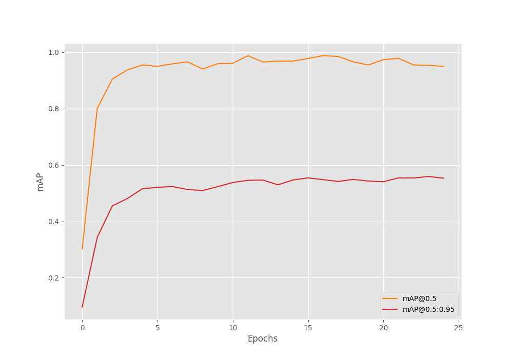
The mAP at 0.50:0.95 IoU seems to be improving pretty much till the end of training. In the last two epochs, the mAP at 0.50 IoU seems to be reducing a bit.

The following is the loss plot for all 25 epochs.

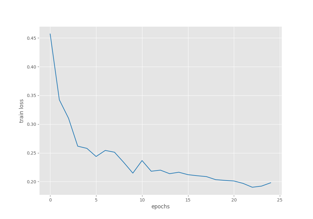
It seems to be increasing in the last two epochs where the mAP was also decreasing.

Inference using the Trained Faster RCNN ResNet50 FPN V2

Now, let’s run inference on some videos. You can run inference using your videos as well and check how the model is performing.

You can use the following command while changing the path to the input video file.

python inference_video.py --weights outputs/training/smoke_detection_fasterrcnn_resnet50_fpn_v2/best_model.pth --input data/inference_data/video_3.mp4 --show-image

The model is doing fairly well here. There is some confusion between the two smoke sources on the right because of which we can see two different detections at the same time.

You may remember that we discussed that smoke detection can be a difficult task for the model to learn properly. Let’s analyze that theory with the following video result.

Clearly, this is a more difficult video compared to the previous one. Here, the model is getting confused about whether it should detect the source of smoke or the emission. Our dataset does not contain such images as well. Therefore, it is not fair to blame the model in this scenario. But this also tells us that building a state-of-the-art smoke detection model will require a much larger dataset.

Faster RCNN ResNet50 FPN V2 vs Faster RCNN ResNet50 FPN

Let’s compare the older Faster RCNN ResNet50 FPN with the newer Faster RCNN ResNet50 FPN V2 model.

Note: The Faster RCNN ResNet50 FPN model was trained using the same configurations for 25 epochs as was in the case of Faster RCNN ResNet50 FPN V2.

For comparison, let’s stack them against each other using the easier video.

It is obvious that the Faster RCNN ResNet50 FPN V2 model is performing much better here. The Faster RCNN ResNet50 FPN model is having multiple false detections.

Summary and Conclusion

In this blog post, we covered the fine tuning process of the Faster RCNN ResNet50 FPN V2 model using PyTorch. We trained it on a smoke detection dataset and also compared it against the Faster RCNN ResNet50 FPN model. The former proved to be better. I hope that this post was helpful to you.

If you have any doubts, thoughts, or suggestions, please leave them in the comment section. I will surely address them.

You can contact me using the Contact section. You can also find me on LinkedIn, and Twitter.

Video Credits Used for Inference

• https://www.youtube.com/watch?v=5_-GB320CBU
• https://www.pexels.com/video/fire-and-smoke-on-fields-13501987/