Steel Surface Defect Detection using Object Detection

Object detection has many real life applications in a lot of industries. Most of the time, in industrial settings, the object detection targets are small. As such, it becomes very difficult to train object detection models effectively. One such problem is steel surface defect detection. Even with deep learning, it is very difficult to tackle the problem with high accuracy. In this article, we will train Faster RCNN object detection models using the PyTorch library.

While doing so, we will analyze how different Faster RCNN object detection models fare against the steel surface defect detection problem. Our primary objective in this article will be to check which model achieves the highest mAP among all that we will train on the steel surface defect detection dataset. Also, it will be important to analyze how large (parameters) the best performing model is.

We will cover the following points in this article:

• We will start with a discussion of the steel surface defect detection dataset.
• After that, we will move on to explore the library that we will use for training the Faster RCNN models on the dataset. This will also include setting up the library locally.
• Then, we will list out all the models that we are going to train on the dataset.
• After training the models, we will analyze the results and use the best model for inference.

The Steel Surface Defect Detection Dataset

To train object detection models for steel surface defect detection, we will need a proper dataset. Fortunately, there is the NEU-DET dataset that we can use.

The dataset contains close-up images of hot-rolled steel strips. Detecting defects in these steel strips is a challenging task. The targets are smaller compared to other datasets. Also, the targets are of various aspects ratios, as we will see later on.

The dataset that we will use here is from Kaggle, the NEU-surface-defect-database. But the original dataset does not contain a training/validation split. So, I created a new dataset with a training/validation split.

You can download the NEU Steel Surface Defect Detect before moving further.

The dataset also contains an accompanying paper, A New Steel Defect Detection Algorithm Based on Deep Learning by Zhao et al. They also try to improve upon the steel surface defect detection technique by modifying a Faster RCNN model and training the model on the dataset.

We are not trying to reproduce the results to compete with their benchmark. Instead, we are trying to carry out our own experiments and figure out the best possible model for the dataset.

If you wish to train the models on your system, please download the dataset before moving further.

Exploring the Steel Surface Detect Detection Dataset

After downloading and extracting the dataset, you should see the following structure.

├── train_annotations [1700 entries exceeds filelimit, not opening dir]
├── train_images [1700 entries exceeds filelimit, not opening dir]
├── valid_annotations [100 entries exceeds filelimit, not opening dir]
└── valid_images [100 entries exceeds filelimit, not opening dir]

The train_images directory contains 1700 images for training and the train_annotations directory contains the corresponding labels.

There are 100 validation images and annotations as well in their respective directories.

The dataset contains 6 different types of steel surface defects. They are:

• crazing
• inclusion
• patches
• pitted_surface
• rolled-in_scale
• scratches

The paper contains the definitions of each of the defect types, in case you need to dive deeper into it.

For now, let’s take a look at a sample image from each class along with the annotations.

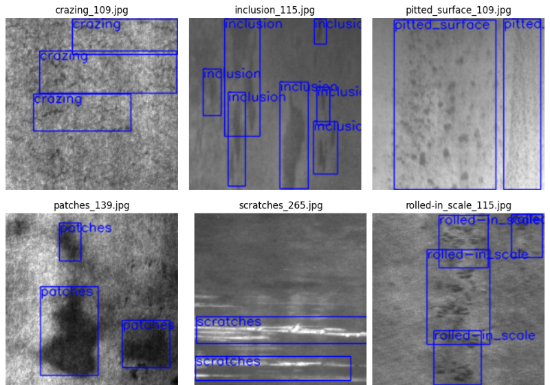
As we can see, the images look like grayscale ones. But they are actually RGB images (3 channels). Also, the aspect ratio of each defect is quite evident from the above images. Each defect has a different shape/aspect ratio. Whatever model we may use, our training strategy will have to be very sound to obtain a high mAP metric on this dataset.

The Faster RCNN Library for Training on the Steel Surface Defect Detection Dataset

We will use the fasterrcnn-pytorch-training-pipeline for experimenting on this dataset. I have been developing this library for quite some time now. It makes training Faster RCNN models a lot easier.

It contains some nice functionalities like auto-logging, an easy-to-use training and inference pipeline, and several Faster RCNN models. In fact, as of now, it contains 27 different Faster RCNN models along with the newest transformer based detection models. They are VitDet and MobileVit based Faster RCNN models.

You can clone the repository and install the requirements if you plan on executing the code yourself.

git clone https://github.com/sovit-123/fasterrcnn-pytorch-training-pipeline.git

For installing the requirements, I first recommend using the Conda command to install PyTorch >= 1.12.0. Then install the rest of the requirements using the following command:

pip install -r requirements.txt

The Project Directory Structure

There are a few more setup details that we need to take a look at. For that, let’s go over the project directory structure.

├── fasterrcnn-pytorch-training-pipeline
│   ├── data
│   ├── data_configs
│   ├── docs
│   ├── example_test_data
│   ├── models
│   ├── notebook_examples
│   ├── outputs
│   ├── __pycache__
│   ├── readme_images
│   ├── torch_utils
│   ├── utils
│   ├── _config.yml
│   ├── datasets.py
│   ├── eval.py
│   ├── inference.py
│   ├── inference_video.py
│   ├── __init__.py
│   ├── README.md
│   ├── requirements.txt
│   └── train.py
└── input
    ├── train_annotations
    ├── train_images
    ├── valid_annotations
    └── valid_images

• In the parent project directory, the input directory contains the dataset that we analyzed earlier.
• All the code that we will execute stays in the fasterrcnn-pytorch-training-pipeline directory that we just cloned above. One of the important directories is the data_configs directory that contains the dataset YAML files (a bit like YOLO YAML files). We will structure this YAML file in the next section.

The YAML file will be provided along with the downloadable zip file that comes with the post. If you need to run training, you just need to clone the repository, download the dataset, and paste the YAML file into the data_configs directory. If you wish to run inference only, you can do so after pasting outputs directory in the fasterrcnn-pytorch-training-pipeline directory. You can find the trained weights here on Kaggle.

Steel Surface Defect Detection using PyTorch and Faster RCNN Models

Now, we will start with the training experiments for steel surface defect detection. We will train three different Faster RCNN models on this dataset.

• ResNet50 FPN V2
• ViTDet
• MobileNetV3 Large FPN

After training, we will use the model with the highest mAP for running inference.

Before we can begin any training experiment, let’s define the dataset YAML file first.

Note: The training experiments were carried out on a system with 10 GB RTX 3080 GPU, 10th generation i7 CPU, and 32 GB of RAM.

Download Code

The Dataset YAML File

We need a dataset YAML file that contains all the dataset configurations. This file goes inside the data_configs directory.

We name it neu_defect.yaml for this project. Following are the contents of the file.

# Images and labels direcotry should be relative to train.py
TRAIN_DIR_IMAGES: '../input/train_images'
TRAIN_DIR_LABELS: '../input/train_annotations'
VALID_DIR_IMAGES: '../input/valid_images'
VALID_DIR_LABELS: '../input/valid_annotations'

# Class names.
CLASSES: [
    '__background__',
    'crazing', 
    'inclusion', 
    'patches',
    'pitted_surface',
    'rolled-in_scale',
    'scratches'
]

# Number of classes (object classes + 1 for background class in Faster RCNN).
NC: 7

# Whether to save the predictions of the validation set while training.
SAVE_VALID_PREDICTION_IMAGES: True

It contains the training and validation directory paths respective to the fasterrcnn-pytorch-training-pipeline directory. Along with that, it contains the class names and the number of classes. The number of classes is equal to the number of object classes in the dataset + the background class.

Faster RCNN ResNet50 FPN V2 Training

Let’s start with training the Faster RCNN ResNet50 FPN V2 on the steel surface defect detection dataset.

Because we have the YAML file and the dataset ready in their respective directories, we can start the training with just one command.

To start the training, execute the following command within the fasterrcnn-pytorch-training-pipeline directory.

python train.py --epochs 20 --data data_configs/neu_defect.yaml --name neu_defect_fasterrcnn_resnet50fpnv2_nomosaic_20e -dw --no-mosaic

We are using a lot of command line arguments above. Let’s go through each of them.

• --epochs: The number of epochs we want to train the model for. We will train each of the models for 20 epochs.
• --data: This accepts the path to the dataset YAML file. For us, it is in the data_configs directory.
• --name: This is the project output directory name. All the training outputs like plots and trained weights will be saved inside outputs/training/{name} directory. In this case, it will be outputs/training/neu_defect_fasterrcnn_resnet50fpnv2_nomosaic_20e. Giving comprehensive names helps to differentiate between multiple directories easily.
• -dw: The repository supports Weights&Biases logging. But passing the -dw command tells the runner script to disable the logging.
• --no-mosaic: The dataset scripts apply mosaic augmentation by default. But here we are disabling them.

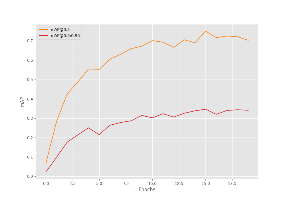
The training will take some time to complete depending on the hardware used. Here are the mAP results from the best epoch.

 Average Precision  (AP) @[ IoU=0.50:0.95 | area=   all | maxDets=100 ] = 0.402
 Average Precision  (AP) @[ IoU=0.50      | area=   all | maxDets=100 ] = 0.724
 Average Precision  (AP) @[ IoU=0.75      | area=   all | maxDets=100 ] = 0.369
 Average Precision  (AP) @[ IoU=0.50:0.95 | area= small | maxDets=100 ] = -1.000
 Average Precision  (AP) @[ IoU=0.50:0.95 | area=medium | maxDets=100 ] = 0.271
 Average Precision  (AP) @[ IoU=0.50:0.95 | area= large | maxDets=100 ] = 0.412
 Average Recall     (AR) @[ IoU=0.50:0.95 | area=   all | maxDets=  1 ] = 0.245
 Average Recall     (AR) @[ IoU=0.50:0.95 | area=   all | maxDets= 10 ] = 0.499
 Average Recall     (AR) @[ IoU=0.50:0.95 | area=   all | maxDets=100 ] = 0.499
 Average Recall     (AR) @[ IoU=0.50:0.95 | area= small | maxDets=100 ] = -1.000
 Average Recall     (AR) @[ IoU=0.50:0.95 | area=medium | maxDets=100 ] = 0.350
 Average Recall     (AR) @[ IoU=0.50:0.95 | area= large | maxDets=100 ] = 0.504

This was after epoch 19. So, it looks like our decision of training the model 20 epochs was good enough. Here, we have the highest mAP of 40.2%.

Analyzing the Faster RCNN ResNet50 FPN V2 Results and Running Evaluation

The following graph shows the mAP plots for IoU at 0.50:0.95 and 0.50.

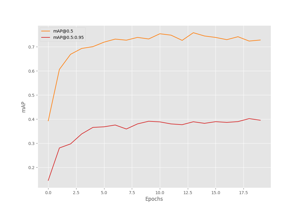
Looks like if we apply some augmentations and train it for longer, then we may achieve even better results.

For now, let’s run the evaluation script on the best model to check the class-wise average precision values.

python eval.py --model fasterrcnn_resnet50_fpn_v2 --weights outputs/training/neu_defect_fasterrcnn_resnet50fpnv2_nomosaic_20e/best_model.pth --data data_configs/neu_defect.yaml --verbose

In the above command, --verbose tells the script to print the class-wise metric.

AP / AR per class
-------------------------------------------------------------------------
|    | Class                | AP                  | AR                  |
-------------------------------------------------------------------------
|1   | crazing              | 0.091               | 0.200               |
|2   | inclusion            | 0.471               | 0.589               |
|3   | patches              | 0.575               | 0.637               |
|4   | pitted_surface       | 0.504               | 0.579               |
|5   | rolled-in_scale      | 0.252               | 0.390               |
|6   | scratches            | 0.518               | 0.600               |
-------------------------------------------------------------------------
|Avg                        | 0.402               | 0.499               |

We have the highest AP for patches and the lowest for the crazing defect.

Training other models will tell us whether these are good numbers or not.

ViTDet Training

Here, we try training a transformer based object detection model on the dataset. This model has a ViT (Vision Transformer) backbone with a Faster RCNN head.

python train.py --model fasterrcnn_vitdet --epochs 20 --data data_configs/neu_defect.yaml --name neu_defect_fasterrcnn_vitdet_nomosaic_20e -dw --no-mosaic --batch 1

The ViTDet model has almost 106 million parameters. So, to fit the training experiment in memory, I had to use a batch size of 1.

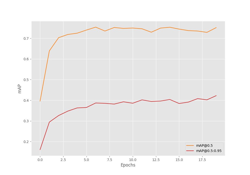
The following block shows the mAP results from the best epoch.

 Average Precision  (AP) @[ IoU=0.50:0.95 | area=   all | maxDets=100 ] = 0.346
 Average Precision  (AP) @[ IoU=0.50      | area=   all | maxDets=100 ] = 0.749
 Average Precision  (AP) @[ IoU=0.75      | area=   all | maxDets=100 ] = 0.293
 Average Precision  (AP) @[ IoU=0.50:0.95 | area= small | maxDets=100 ] = -1.000
 Average Precision  (AP) @[ IoU=0.50:0.95 | area=medium | maxDets=100 ] = 0.210
 Average Precision  (AP) @[ IoU=0.50:0.95 | area= large | maxDets=100 ] = 0.354
 Average Recall     (AR) @[ IoU=0.50:0.95 | area=   all | maxDets=  1 ] = 0.212
 Average Recall     (AR) @[ IoU=0.50:0.95 | area=   all | maxDets= 10 ] = 0.487
 Average Recall     (AR) @[ IoU=0.50:0.95 | area=   all | maxDets=100 ] = 0.518
 Average Recall     (AR) @[ IoU=0.50:0.95 | area= small | maxDets=100 ] = -1.000
 Average Recall     (AR) @[ IoU=0.50:0.95 | area=medium | maxDets=100 ] = 0.367
 Average Recall     (AR) @[ IoU=0.50:0.95 | area= large | maxDets=100 ] = 0.520

This was after epoch 16. The result of ViTDet is very interesting. We can see that mAP at IoU 0.50 is higher than the Faster RCNN ResNetFPN V2 fine tuning. But the mAP for IoU at 0.50:0.95 is lower.

Analyzing the ViTDet Results and Running Evaluation

The following figure shows the mAP plots for the ViTDet Training.

We can see some indications of overfitting. Looks like the ViTDet model can surely help by using some augmentations.

The following blocks show the code for running the evaluation and the results.

python eval.py --weights outputs/training/neu_defect_fasterrcnn_vitdet_nomosaic_20e/best_model.pth --model fasterrcnn_vitdet --data data_configs/neu_defect.yaml --verbose --batch 4

-------------------------------------------------------------------------
|    | Class                | AP                  | AR                  |
-------------------------------------------------------------------------
|1   | crazing              | 0.077               | 0.361               |
|2   | inclusion            | 0.394               | 0.543               |
|3   | patches              | 0.450               | 0.588               |
|4   | pitted_surface       | 0.450               | 0.610               |
|5   | rolled-in_scale      | 0.218               | 0.429               |
|6   | scratches            | 0.491               | 0.578               |
-------------------------------------------------------------------------
|Avg                        | 0.347               | 0.518               |

Here also, the average precision results follow a similar trend to the Faster RCNN ResNet50 FPN V2 training. We have the lowest AP for crazing and the highest for patches & pitted_surface.

Faster RCNN MobileNetV3 Large FPN Training

We will run a final training experiment on the steel surface defect detection dataset using the Faster RCNN MobileNetV3 Large FPN model.

python train.py --model fasterrcnn_mobilenetv3_large_fpn --epochs 20 --data data_configs/neu_defect.yaml --name neu_defect_fasterrcnn_mobilenetv3_large_fpn_nomosaic_20e -dw --no-mosaic --batch 16

 Average Precision  (AP) @[ IoU=0.50:0.95 | area=   all | maxDets=100 ] = 0.422
 Average Precision  (AP) @[ IoU=0.50      | area=   all | maxDets=100 ] = 0.752
 Average Precision  (AP) @[ IoU=0.75      | area=   all | maxDets=100 ] = 0.440
 Average Precision  (AP) @[ IoU=0.50:0.95 | area= small | maxDets=100 ] = -1.000
 Average Precision  (AP) @[ IoU=0.50:0.95 | area=medium | maxDets=100 ] = 0.320
 Average Precision  (AP) @[ IoU=0.50:0.95 | area= large | maxDets=100 ] = 0.427
 Average Recall     (AR) @[ IoU=0.50:0.95 | area=   all | maxDets=  1 ] = 0.266
 Average Recall     (AR) @[ IoU=0.50:0.95 | area=   all | maxDets= 10 ] = 0.504
 Average Recall     (AR) @[ IoU=0.50:0.95 | area=   all | maxDets=100 ] = 0.504
 Average Recall     (AR) @[ IoU=0.50:0.95 | area= small | maxDets=100 ] = -1.000
 Average Recall     (AR) @[ IoU=0.50:0.95 | area=medium | maxDets=100 ] = 0.349
 Average Recall     (AR) @[ IoU=0.50:0.95 | area= large | maxDets=100 ] = 0.510

Here, we get the best mAP on epoch 20. And surprisingly, this is the best performing model. We have the highest mAP of 42.2% among all the three models in this case.

This is surprising because it is the smallest model among the three. One reason can be that we use a higher batch size for this experiment. Because of this, batch normalization could be behaving better compared to the above two experiments.

Analyzing the Faster RCNN MobileNetV3 Large FPN Results and Running Evaluation

Here is the mAP graph for training the Faster RCNN MobileNetV3 Large FPN model on the steel surface defect detection dataset.

It looks like training for longer may give is even higher mAP in this case.

The following blocks run the evaluation and show the results.

python eval.py --weights outputs/training/neu_defect_fasterrcnn_mobilenetv3_large_fpn_nomosaic_20e/best_model.pth --model fasterrcnn_mobilenetv3_large_fpn --data data_configs/neu_defect.yaml --verbose

AP / AR per class
-------------------------------------------------------------------------
|    | Class                | AP                  | AR                  |
-------------------------------------------------------------------------
|1   | crazing              | 0.135               | 0.255               |
|2   | inclusion            | 0.452               | 0.575               |
|3   | patches              | 0.561               | 0.617               |
|4   | pitted_surface       | 0.570               | 0.624               |
|5   | rolled-in_scale      | 0.257               | 0.361               |
|6   | scratches            | 0.557               | 0.600               |
-------------------------------------------------------------------------
|Avg                        | 0.422               | 0.505               |

In this case, we have the highest average precision for the pitted_surface class.

Running Inference on the Steel Surface Defect Detection

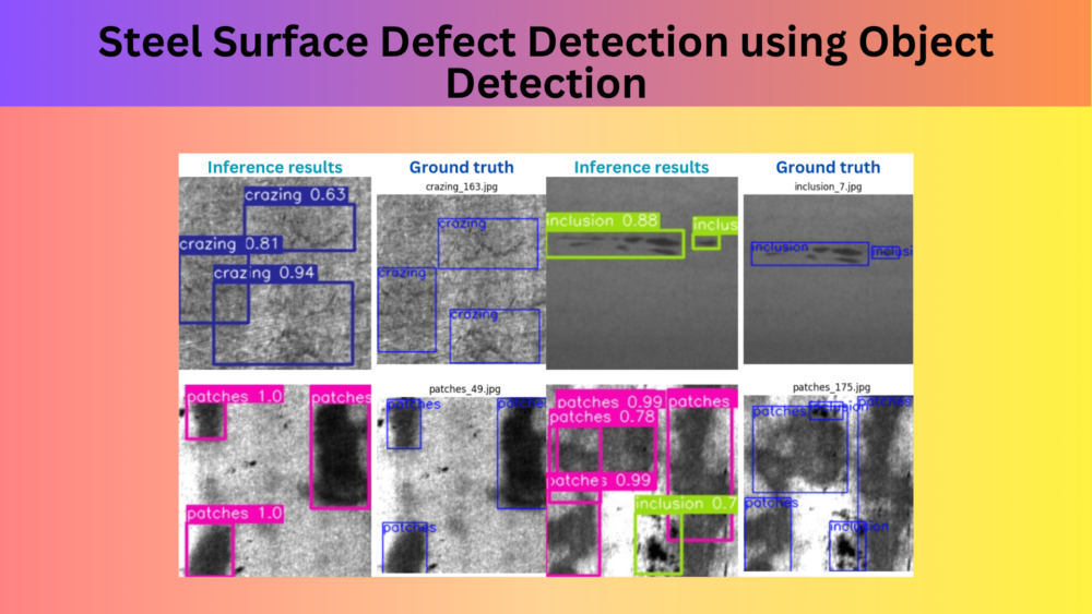
We don’t have separate unseen images for this dataset. So, we will use the validation images for running inference. We will use the best Faster RCNN MobileNetV3 Large FPN weights for this. Also, we will compare a few results with the ground truth.

The following command runs the inference on all the validation images.

python inference.py --weights outputs/training/neu_defect_fasterrcnn_mobilenetv3_large_fpn_nomosaic_20e/best_model.pth --input ../input/valid_images/ --threshold 0.5

Here are some comparisons where the inference and the ground truth have a good match.

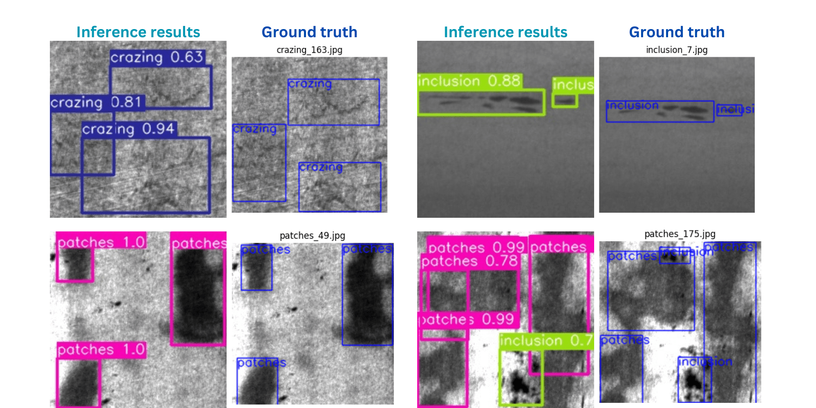
The model is also able to detect the patches along with the inclusion defect in one of the images.

Now, let’s take a look at some of the results which are not perfect.

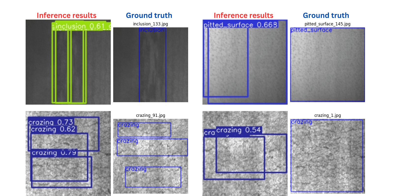
As we can see, in most cases, the model is detecting multiple defects where there is only one defect.

Further Improvements

We can carry out the following experiments to try to increase the accuracy of the models:

• Using augmentations while training. With this repository, using the --use-train-aug flag applies augmentations.
• Training with even higher resolution images using the --imgsz flag may also help.

Summary and Conclusion

In this article, we tried to tackle a real life application using deep learning. We trained several object detection models on the steel surface defect detection dataset. After training, we used the best model for analyzing the results even further to know where the model makes the mistakes. If you work on further improving the results, try to post your findings in the comment section. I hope that this article was useful to you.

If you have doubts, thoughts, or suggestions, please leave them in the comment section. I will surely address them.

You can contact me using the Contact section. You can also find me on LinkedIn, and Twitter.