
Twitter has become mainstream nowadays, both as a social media and a communication platform. People use it for various purposes, including real-time tweets about accidents and disasters. But a lot of times it is not clear whether the tweet is actually about an accident/disaster or not. A deep learning model which can classify tweets can surely help here. As such, in this article, we will build an NLP model using PyTorch for disaster tweet classification.
Deep learning based natural language processing models can help solve many real-world problems. Building a model which can classify whether a tweet is about a disaster or not in real-time can help notify the rightful authorities. Of course, there are many other components involved in building such a system. But here, let’s just focus on building the deep learning model which can carry out disaster tweet classification.

Here are all the points that we will cover in this tutorial:
- We will start by exploring the tweet classification dataset. This dataset is part of a playground competition on Kaggle.
- Then we will move on to the coding part. This involves:
- The dataset preparation.
- The model preparation.
- Training and validation by splitting the training set of the original dataset.
- And finally carrying out inference on the test set.
In the previous post, we started exploring NLP for text classification using Deep Learning with a code-first approach. There we used a simple model to classify movie reviews as positive or negative. This article will not be much different than that. The dataset is in CSV format in this case. And the tweet lengths are smaller compared to the lengthy movie reviews. This will help us reinforce the concepts of text classification using deep learning.
The Disaster Tweet Classification Dataset
We will use the dataset from one of the “Getting Started” competitions from Kaggle. It is the Natural Language Processing with Disaster Tweets dataset.
This dataset is just perfect to start learning about deep learning based NLP. It contains real tweets which may either be related to a natural disaster or not. Monitoring such tweets can help relief organizations and news agencies to act faster in case of a real disaster.
But it is very difficult for machines (and sometimes for humans as well) to tell right away which tweets are about disasters happening at the current moment in a place.
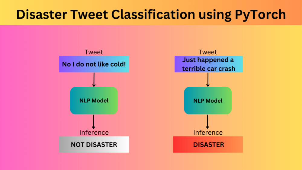
For this, we can train a deep learning model which can classify the tweets as either DISASTER or NOT DISASTER.
For example, take a look at the following tweet.
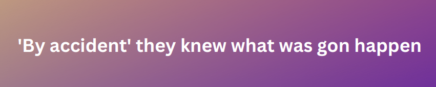
The tweet contains the word “accident” but is not actually about any major accident happening in real time. So, it is not actually a disaster. It is slightly confusing for us also to figure that out. And machine learning models cannot do it right away without proper training.
There are many more confusing tweets in the dataset. And the best way is to build a deep learning based NLP model for disaster tweet classification which can classify such tweets in real-time.
The Dataset Format
For now, please go ahead and download the dataset from Kaggle.
After extracting it, you should get the following directory structure.
├── sample_submission.csv
├── test.csv
└── train.csv
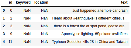
There are three CSV files. The train.csv file contains the training set along with the ground truth labels. Here is an image showing a few samples from the training CSV file.
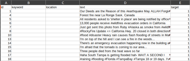
We are most interested in the text and target columns. They contain the tweet and the target label respectively. If the tweet is actually about a disaster, the target value is 1, else it is 0.
The training CSV contains 7614 samples.
As it is a competition dataset, we also have an unlabeled test.csv file. This is the file that one needs to run the prediction on after training the model and then store the results in the submission.csv file for submission. But we will not carry out these steps.
We will split the train.csv files into a training and validation sample for training our deep learning NLP model.
The Disaster Tweet Classification Project Directory Structure
Before moving any further, let’s check the entire directory structure.
.
├── input
│   ├── sample_submission.csv
│   ├── test.csv
│   └── train.csv
├── outputs
│   └── simple_embedding
│       ├── accuracy.png
│       ├── loss.png
│       └── model.pth
└── disaster_tweet_classification_simple_embedding.ipynb
- The
inputdirectory contains the dataset as we discussed above. - The
outputsdirectory contains the trained model and the accuracy and loss graphs. - And the project root directory contains a Jupyter Notebook with all the code.
The trained model along with the notebook will be available via the downloadable zip file that comes with this article.
Note: A lot of code and functions are very similar to the previous post. The only changes will be considering that in the previous post, we had text files and here we have a CSV file. We will go through each code block, but for detailed explanations, please refer to the previous post.
PyTorch Version
Any version of PyTorch >= 1.11.0 should work perfectly for this project.
Disaster Tweet Classification Using Deep Learning
From here on, we will start exploring the code as present in the Jupyter Notebook. Let’s start with the import statements, setting the working directories, and setting the seed for reproducibility across runs.
Download Code
import torch
import os
import pathlib
import numpy as np
import string
import re
import glob
import torch.nn as nn
import torch.nn.functional as F
import torch.optim as optim
import matplotlib.pyplot as plt
import pandas as pd
import random

from tqdm.auto import tqdm
from collections import Counter
from torch.utils.data import DataLoader, Dataset, Subset

plt.style.use('ggplot')
# Set seed.
seed = 42
np.random.seed(seed)
torch.manual_seed(seed)
torch.cuda.manual_seed(seed)
torch.backends.cudnn.deterministic = True
torch.backends.cudnn.benchmark = True
OUTPUTS_DIR = os.path.join('outputs', 'simple_embedding')
os.makedirs(OUTPUTS_DIR, exist_ok=True)
dataset_dir = os.path.join('input')
print(os.listdir(dataset_dir))
In the above code block, we define the:
dataset_dir: This is theinputdirectory holding the CSV files.OUTPUTS_DIR: All the outputs will be stored in theoutputs/simple_embeddingdirectory.
Preparing the Disaster Tweet Classification Dataset
Let’s start focusing on preparing the disaster tweet classification dataset. This is going to be one of the most important parts of the entire project.
We will start with reading the training and test CSV files.
data_train = pd.read_csv(os.path.join(dataset_dir, 'train.csv'))
data_train.head()
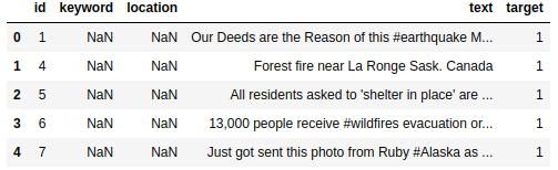
data_test = pd.read_csv(os.path.join(dataset_dir, 'test.csv'))
data_test.head()
train_tweets = data_train.text
train_targets = data_train.target

test_tweets = data_test.text

print(f"Number of training samples: {len(train_tweets)}")
print(f"Number of test samples: {len(test_tweets)}")
Here are the outputs of the above code cell.
Number of training samples: 7613
Number of test samples: 3263
There are 7613 training samples and 3263 test samples. We will spit a part of the current training samples to create the validation set.
Finding the Longest Tweet and Average Length of All Tweets
The following function helps us find the number of words in the longest tweet.
def find_longest_length(tweets):
    """
    Find the longest tweet in the entire training set.

    :param tweets: A pandas data series.

    Returns:
        max_length: Longest tweet length.
    """
    max_length = 0
    for i, text in enumerate(tweets):
        corpus = [
            word for word in text.split()
        ]
        if len(corpus) > max_length:
            max_length = len(corpus)
    return max_length
Please note that we do not do any cleaning in the above function. It compares the lengths of all the tweets directly from the CSV file.
longest_sentence_length = find_longest_length(train_tweets)
print(f"Longest tweet: {longest_sentence_length} words")
We pass the train_tweets Series to the function and get the following output.
Longest tweet: 31 words
The longest tweet contains 31 words.
Next, we will find the average length of all the tweets.
def find_avg_sentence_length(tweets):
    """
    Find the average sentence length among all
    the tweets.

    :param tweets: A pandas data series.

    Returns:
        Average sentence length.
    """
    sentence_lengths = []
    for i, text in enumerate(tweets):
        corpus = [
                word for word in text.split()
            ]
        sentence_lengths.append(len(corpus))
    return sum(sentence_lengths)/len(sentence_lengths)
Calling the function and printing the output.
average_length = find_avg_sentence_length(train_tweets)
print(f"Average sentence length: {average_length} words")
Average sentence length: 14.903585971364771 words
The average sentence length considering all the tweets is 14.9. This is important for the next part.
We need to define some constants before moving further in the coding part.
MAX_LEN = int(longest_sentence_length)
# Use these many top words from the dataset. If -1, use all words.
NUM_WORDS = -1 # Vocabulary size.
# Batch size.
BATCH_SIZE = 512
VALID_SPLIT = 0.20
Going over all the constants defined in the above block:
MAX_LEN: This is the maximum length of a tweet that we will consider while preparing the dataset. If the tweet is longer than this length, then it will be truncated, and if shorter, we will pad it with 0s.NUM_WORDS: This defines the number of words that we will consider from the entire dataset to create the vocabulary of the dataset. -1 will retain all the unique words from the datasets for creating the vocabulary.BATCH_SIZE: The batch size for the data loaders.VALID_SPLIT: We are using 20% of the data for validation and the rest for training.
Helper Functions for Dataset Preparation
We need to find the number of occurrences of each unique word in the dataset. For that, we write a find_word_frequency function.
def find_word_frequency(tweets, most_common=None):
    """
    Create a list of tuples of the following format,
    [('ho', 2), ('hello', 1), ("let's", 1), ('go', 1)]
    where the number represents the frequency of occurance of
    the word in the entire dataset.

    :param tweets: A pandas data series.
    :param most_common: Return these many top words from the dataset.
        If `most_common` is None, return all. If `most_common` is 3,
        returns the top 3 tuple pairs in the list.

    Returns:
        sorted_words: A list of tuple containing each word and it's
        frequency of the format ('ho', 2), ('hello', 1), ...]
    """
    # Add all the words in the entire dataset to `corpus` list.
    corpus = []
    for i, text in enumerate(tweets):
            corpus.extend([
                word for word in text.split()
            ])
    count_words = Counter(corpus)
    # Create a dictionary with the most common word in the corpus
    # at the beginning.
    # `word_frequency` will be like
    word_frequency = count_words.most_common(n=most_common) # Returns all if n is `None`.
    return word_frequency
The above function returns a dictionary where the keys contain each of the unique words and the values are the number of occurrences in the dataset. They are arranged in descending order of occurrence. So, the word with the highest occurrence in the dataset will be the first element in the dictionary.
We need to assign an integer value to each unique word before so that the neural network can process them. We have a word2int function for that.
def word2int(input_words, num_words):
    """
    Create a dictionary of word to integer mapping for each unique word.

    :param input_words: A list of tuples containing the words and
        theiry frequency. Should be of the following format,
        [('ho', 2), ('hello', 1), ("let's", 1), ('go', 1)]
    :param num_words: Number of words to use from the `input_words` list
        to create the mapping. If -1, use all words in the dataset.

    Returns:
        int_mapping: A dictionary of word and a integer mapping as
            key-value pair. Example, {'Hello,': 1, 'the': 2, 'let': 3}
    """

    if num_words > -1:
        int_mapping = {
            w:i+1 for i, (w, c) in enumerate(input_words) \
                if i <= num_words - 1 # -1 to avoid getting (num_words + 1) integer mapping.
        }
    else:
        int_mapping = {w:i+1 for i, (w, c) in enumerate(input_words)}
    return int_mapping
This function also returns a dictionary where the value will be a unique integer starting from 1. We reserve the integer 0 for padding the vectors later on.
The Custom Dataset Class
The following code block contains the entire custom dataset class.
class NLPClassificationDataset(Dataset):
    def __init__(self, tweets, labels, word_frequency, int_mapping, max_len):
        self.word_frequency = word_frequency
        self.int_mapping = int_mapping
        self.tweets = tweets
        self.labels = labels
        self.max_len = max_len

    def standardize_text(self, input_text):
        # Convert everything to lower case.
        text = input_text.lower()
        # Remove punctuation marks using `string` module.
        # According to `string`, the following will be removed,
        # '!"#$%&\'()*+,-./:;<=>?@[\\]^_`{|}~'
        text = ''.join([
            character for character in text \
                if character not in string.punctuation
        ])
        return text

    def return_int_vector(self, int_mapping, tweet):
        """
        Assign an integer to each word and return the integers in a list.
        """
        text = self.standardize_text(tweet)
        corpus = [
            word for word in text.split()
        ]
        # Each word is replaced by a specific integer.
        int_vector = [
            int_mapping[word] for word in text.split() \
            if word in int_mapping
        ]
        return int_vector

    def pad_features(self, int_vector, max_len):
        """
        Return features of `int_vector`, where each vector is padded
        with 0's or truncated to the input seq_length. Return as Numpy
        array.
        """
        features = np.zeros((1, max_len), dtype = int)
        if len(int_vector) <= max_len:
            zeros = list(np.zeros(max_len - len(int_vector)))
            new = zeros + int_vector
        else:
            new = int_vector[: max_len]
        features = np.array(new)
        return features

    def __len__(self):
        return len(self.tweets)

    def __getitem__(self, idx):
        tweet = self.tweets[idx]
        int_vector = self.return_int_vector(self.int_mapping, tweet)
        padded_features = self.pad_features(int_vector, self.max_len)
        label = self.labels[idx]
        return {
            'text': torch.tensor(padded_features, dtype=torch.int32),
            'label': torch.tensor(label, dtype=torch.long)
        }
The above dataset class covers the following steps:
- Firstly, it converts all the tweets into an integer vector based in the
word2intmapping. While doing so, it cleans the text as well. As simple natural language processing neural networks are not good with special symbols, it is better to remove them for now. There are a lot of “@” tags that we surely need to remove. - Secondly, it pads the shorter (less than 31 integers/words) vectors with 0s to the left.
- Finally, we return a dictionary where the
textkey contains the converted tweet tensor and thelabelkey the corresponding label.
There are some other details in the above class as well. In case you need it, feel free to go through it before moving forward.
Finding the Word Frequency and Preparing the Data Loaders
Let’s find the frequency of each word that we need for initializing the above dataset class.
# Get the frequency of all unqiue words in the dataset.
word_frequency = find_word_frequency(train_tweets)
# Assign a specific intenger to each word.
int_mapping = word2int(word_frequency, num_words=NUM_WORDS)

print(len(int_mapping))
We get the following output after executing the above block.
31924
So, there are 31924 unique words in the entire dataset.
Now, we can create the training and validation dataset.
dataset = NLPClassificationDataset(
    train_tweets, train_targets, word_frequency, int_mapping, MAX_LEN
)

dataset_size = len(dataset)
# Calculate the validation dataset size.
valid_size = int(VALID_SPLIT*dataset_size)
# Radomize the data indices.
indices = torch.randperm(len(dataset)).tolist()
# Training and validation sets.
dataset_train = Subset(dataset, indices[:-valid_size])
dataset_valid = Subset(dataset, indices[-valid_size:])

# dataset_valid = NLPClassificationDataset()
print(f"Number of training samples: {len(dataset_train)}")
print(f"Number of validation samples: {len(dataset_valid)}")
Number of training samples: 6091
Number of validation samples: 1522
According to the split that we use, there are 6091 training samples and 1522 validation samples.
It is better if we can visualize a few samples from the created dataset. Let’s create an integer-to-word mapping and convert a few samples to do a sanity check.
# Integer to word mapping for the training dataset.
int2word_train = {value: key for key, value in int_mapping.items()}

# Print a few samples input and its label.
for i in range(10):
    rand_num = random.randint(0, 6000)
    inputs = ''
    for x in dataset_train[rand_num]['text']:
        if x != 0:
            inputs += ' ' + int2word_train[int(x)]
    print(inputs)
    if int(dataset_train[rand_num]['label']) == 1:
        label = 'DISASTER'
    else:
        label = 'NOT_DISASTER'
    print('LABEL:', label)
    print('#'*25)
Here are 10 converted samples along with their labels.
 there is no greater tragedy than becoming comfortable with where you are in life
LABEL: NOT_DISASTER
#########################
 feel like his movies have done more harm than good they make us look sterotypical annddd colorism is prevalent sort of
LABEL: NOT_DISASTER
#########################
 oil spill may have been costlier bigger than projected a all oil spill off
LABEL: DISASTER
#########################
 news families to sue over more than 40 families affected by the fatal outbreak of
LABEL: DISASTER
#########################
 us wants future first responders to be more
LABEL: NOT_DISASTER
#########################
 war patch us 71st evacuation hospital
LABEL: DISASTER
#########################
 stock market crash are there in the rubble
LABEL: DISASTER
#########################
 wildfire burns on california us economic net
LABEL: DISASTER
#########################
 galactic crash early unlocking of brakes triggered structural failure
LABEL: DISASTER
#########################
 what do you take me for im not a mass murderer just the one
LABEL: NOT_DISASTER
#########################
As we can see, all the special symbols have been removed from the final dataset.
For the final part of the data preparation, we create the training and validation data loaders.
train_loader = DataLoader(
    dataset_train,
    batch_size=BATCH_SIZE,
    shuffle=True,
    num_workers=4
)

valid_loader = DataLoader(
    dataset_valid,
    batch_size=BATCH_SIZE,
    shuffle=False,
    num_workers=4
)
This completes the dataset preparation part.
Binary Accuracy Metrics, Training, and Validation Functions
We will use the binary accuracy metric for evaluating the disaster tweet classification model. The following block contains the code for it.
def binary_accuracy(labels, outputs, train_running_correct):
    # As the outputs are currently logits.
    outputs = torch.sigmoid(outputs)
    running_correct = 0
    for i, label in enumerate(labels):
        if label < 0.5 and outputs[i] < 0.5:
            running_correct += 1
        elif label >= 0.5 and outputs[i] >= 0.5:
            running_correct += 1
    return running_correct
As the outputs from the models are logits, we first pass them through the Sigmoid function. The running_correct variable keeps track of how many samples are correctly classified by the model.
Next, we need the training and validation functions.
# Training function.
def train(model, trainloader, optimizer, criterion, device):
    model.train()
    print('Training')
    train_running_loss = 0.0
    train_running_correct = 0
    counter = 0
    for i, data in tqdm(enumerate(trainloader), total=len(trainloader)):
        counter += 1
        inputs, labels = data['text'], data['label']
        inputs = inputs.to(device)
        labels = torch.tensor(labels, dtype=torch.float32).to(device)
        optimizer.zero_grad()
        # Forward pass.
        outputs = model(inputs)
        outputs = torch.squeeze(outputs, -1)
        # Calculate the loss.
        loss = criterion(outputs, labels)
        train_running_loss += loss.item()
        running_correct = binary_accuracy(
            labels, outputs, train_running_correct
        )
        train_running_correct += running_correct
        # Backpropagation.
        loss.backward()
        # Update the optimizer parameters.
        optimizer.step()

    # Loss and accuracy for the complete epoch.
    epoch_loss = train_running_loss / counter
    epoch_acc = 100. * (train_running_correct / len(trainloader.dataset))
    return epoch_loss, epoch_acc

# Validation function.
def validate(model, testloader, criterion, device):
    model.eval()
    print('Validation')
    valid_running_loss = 0.0
    valid_running_correct = 0
    counter = 0

    with torch.no_grad():
        for i, data in tqdm(enumerate(testloader), total=len(testloader)):
            counter += 1
            inputs, labels = data['text'], data['label']
            inputs = inputs.to(device)
            labels = torch.tensor(labels, dtype=torch.float32).to(device)
            # Forward pass.
            outputs = model(inputs)
            outputs = torch.squeeze(outputs, -1)
            # Calculate the loss.
            loss = criterion(outputs, labels)
            valid_running_loss += loss.item()
            running_correct = binary_accuracy(
                labels, outputs, valid_running_correct
            )
            valid_running_correct += running_correct

    # Loss and accuracy for the complete epoch.
    epoch_loss = valid_running_loss / counter
    epoch_acc = 100. * (valid_running_correct / len(testloader.dataset))
    return epoch_loss, epoch_acc
As usual, backpropagation happens during training only. We return the loss and accuracy values from both functions.
The Deep Learning Model
Just like in the case of movie review classification, here also, we define a simple model with one embedding layer and one linear layer.
 class SimpleEmbedding(nn.Module):
    def __init__(self, vocab_size, max_len, embed_dim):
        super(SimpleEmbedding, self).__init__()
        self.embedding = nn.Embedding(vocab_size, embedding_dim=embed_dim)
        self.linear1 = nn.Linear(max_len, 1)

        self.dropout = nn.Dropout(0.5)

    def forward(self, x):
        x = self.embedding(x)
        x = self.dropout(x)
        bs, _, _ = x.shape
        x = F.adaptive_avg_pool1d(x, 1).reshape(bs, -1)
        out = self.linear1(x)
        return out
Now, define the computation device and initialize the model.
device = torch.device('cuda' if torch.cuda.is_available() else 'cpu')
print(device)

EMBED_DIM = 50
model = SimpleEmbedding(
    len(int_mapping)+1,
    MAX_LEN,
    EMBED_DIM
).to(device)
We are using an embedding dimension of 50 for now.
Training the Model on the Disaster Tweet Classification Dataset
Before training the mode, we need to define the optimizer and the loss function. We do that in the next code block.
print(model)
criterion = nn.BCEWithLogitsLoss()
optimizer = optim.Adam(
    model.parameters(),
    lr=0.001,
)
# Total parameters and trainable parameters.
total_params = sum(p.numel() for p in model.parameters())
print(f"{total_params:,} total parameters.")
total_trainable_params = sum(
    p.numel() for p in model.parameters() if p.requires_grad)
print(f"{total_trainable_params:,} training parameters.\n")
The model contains approximately 1.6 million trainable parameters.
Finally, we get to the training loop.
epochs = 125
# Lists to keep track of losses and accuracies.
train_loss, valid_loss = [], []
train_acc, valid_acc = [], []
# Start the training.
for epoch in range(epochs):
    print(f"[INFO]: Epoch {epoch+1} of {epochs}")
    train_epoch_loss, train_epoch_acc = train(model, train_loader,
                                            optimizer, criterion, device)
    valid_epoch_loss, valid_epoch_acc = validate(model, valid_loader,
                                                criterion, device)
    train_loss.append(train_epoch_loss)
    valid_loss.append(valid_epoch_loss)
    train_acc.append(train_epoch_acc)
    valid_acc.append(valid_epoch_acc)
    print(f"Training loss: {train_epoch_loss}, training acc: {train_epoch_acc}")
    print(f"Validation loss: {valid_epoch_loss}, validation acc: {valid_epoch_acc}")

    # Save model.
    torch.save(
        model, os.path.join(OUTPUTS_DIR, 'model.pth')
    )
    print('-'*50)
We are training the model for 125 epochs and printing the loss and binary accuracy value after each epoch.
Here are some of the truncated outputs.
[INFO]: Epoch 1 of 125
Training
100%
12/12 [00:00<00:00, 18.55it/s]
Validation
100%
3/3 [00:00<00:00, 24.84it/s]
Training loss: 0.6854898830254873, training acc: 56.37826301099984
Validation loss: 0.6837570667266846, validation acc: 57.3587385019711
--------------------------------------------------
.
.
.
[INFO]: Epoch 125 of 125
Training
100%
12/12 [00:00<00:00, 32.36it/s]
Validation
100%
3/3 [00:00<00:00, 26.90it/s]
Training loss: 0.29964092125495273, training acc: 87.98226892135939
Validation loss: 0.5089770754178365, validation acc: 76.87253613666229
--------------------------------------------------
After the final epoch, the model achieves a validation accuracy of 76.87%. This may not be great but is not too bad either. Remember that we have only around 6000 training samples and a very simple model with 1.6 million trainable parameters. In such circumstances, we can safely say that the model is performing fairly well.
The Accuracy and Loss Plots
Here is the code to plot the accuracy and loss graphs and also to save these to the disk.
def save_plots(train_acc, valid_acc, train_loss, valid_loss):
    """
    Function to save the loss and accuracy plots to disk.
    """
    # Accuracy plots.
    plt.figure(figsize=(10, 7))
    plt.plot(
        train_acc, color='blue', linestyle='-',
        label='train accuracy'
    )
    plt.plot(
        valid_acc, color='red', linestyle='-',
        label='validataion accuracy'
    )
    plt.xlabel('Epochs')
    plt.ylabel('Accuracy')
    plt.legend()
    plt.savefig(os.path.join(OUTPUTS_DIR, 'accuracy.png'))
    plt.show()
    # Loss plots.
    plt.figure(figsize=(10, 7))
    plt.plot(
        train_loss, color='blue', linestyle='-',
        label='train loss'
    )
    plt.plot(
        valid_loss, color='red', linestyle='-',
        label='validataion loss'
    )
    plt.xlabel('Epochs')
    plt.ylabel('Loss')
    plt.legend()
    plt.savefig(os.path.join(OUTPUTS_DIR, 'loss.png'))
    plt.show()

save_plots(train_acc, valid_acc, train_loss, valid_loss)
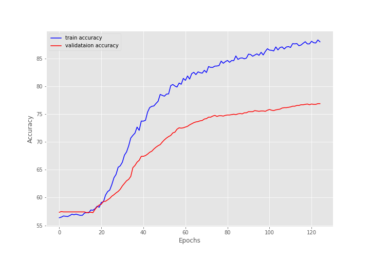
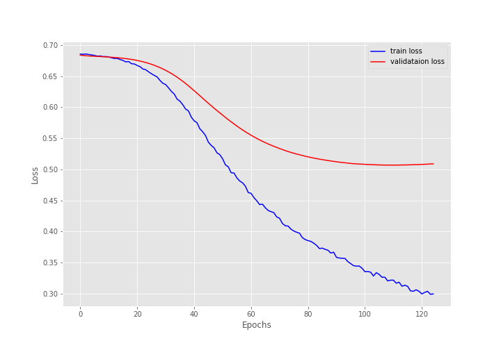
The training plots for both accuracy and loss look pretty good. But the validation loss seems to be increasing after 120 epochs. This indicates overfitting. Training any longer would have given us a considerably more overfit model.
Inference on Unseen Tweets for Disaster Classification
For inference, we will use two tweets from the test set. One of them is a disaster tweet and one is not. First, we need to load the trained model from the disk.
trained_model = torch.load(
    os.path.join(OUTPUTS_DIR, 'model.pth')
)
Then, we need to define a list containing two tweets from the test set.
# A few real-life tweets taken from the test set.
sentences = [
    'No I do not like cold!',
    'Just happened a terrible car crash'
]
The first tweet is not a disaster but the second one is.
Let’s redefine two functions to convert text to integer and pad the integer vectors. This is necessary because we do not have access to the dataset class during inference.
def return_int_vector(int_mapping, text):
        """
        Assign an integer to each word and return the integers in a list.
        """
        corpus = [
            word for word in text.split()
        ]
        # Each word is replaced by a specific integer.
        int_vector = [
            int_mapping[word] for word in text.split() \
            if word in int_mapping
        ]
        return int_vector

def pad_features(int_vector, max_len):
    """
    Return features of `int_vector`, where each vector is padded
    with 0's or truncated to the input seq_length. Return as Numpy
    array.
    """
    features = np.zeros((1, max_len), dtype = int)
    if len(int_vector) <= max_len:
        zeros = list(np.zeros(max_len - len(int_vector)))
        new = zeros + int_vector
    else:
        new = int_vector[: max_len]
    features = np.array(new)
    return features
Finally, we can loop over the tweets and run the inference.
for sentence in sentences:
    int_vector = return_int_vector(int_mapping, sentence)
    padded_features = pad_features(int_vector, int(longest_sentence_length))
    input_tensor = torch.tensor(padded_features, dtype=torch.int32)
    input_tensor = input_tensor.unsqueeze(0)
    with torch.no_grad():
        output = model(input_tensor.to(device))
    preds = torch.sigmoid(output)
    print(sentence)
    print(f"Prediction score: {preds.cpu().numpy()}")
    if preds > 0.5:
        print('Prediction: DISASTER')
    else:
        print('Prediction: NOT_DISASTER')
    print('\n')
This is the output that we get.
No I do not like cold!
Prediction score: [[0.23451447]]
Prediction: NOT_DISASTER


Just happened a terrible car crash
Prediction score: [[0.6955336]]
Prediction: DISASTER
The model is able to classify the tweets correctly. It classifies the second one as a disaster tweet with 69.5% accuracy and the first one as not a disaster tweet with 76.5% accuracy. This is pretty good.
Next Steps for the Disaster Tweet Classification Project
In case you are interested in improving the validation results even more, there are a few approaches you can consider.
- Using pretrained Roberta models from Torchtext.
- Using Huggingface transformers.
We will also cover the above two topics in future articles.
Summary and Conclusion
In this article, we covered a simple NLP project on disaster tweet classification using deep learning. We prepared the dataset from one of the Kaggle playground competitions, cleaned it, and fed it to a simple embedding model for training. After training, we also carried out inference. Such a model in itself is not very useful at all. It needs to have other components such as finding out the location of the tweet in case there is actually a disaster. Then it needs to send the information to the appropriate authority. But this is the first step for such a complete project. I hope that this article was worth your time.
If you have doubts, thoughts, or suggestions, please leave them in the comment section. I will surely address them.
You can contact me using the Contact section. You can also find me on LinkedIn, and X.

2 thoughts on “Disaster Tweet Classification using PyTorch”