Getting Started with Text Classification using Pytorch, NLP, and Deep Learning

Starting Natural Language Processing (NLP) can be confusing at times. Especially, for someone coming from the field of Computer Vision. Further, in 2023 there are just a million resources out there to start learning NLP. With all the resources revolving around transformers and methods which came before, the process can easily become overwhelming. But we can make it a bit easier. In this article, we will start with text classification using NLP. And this most probably it is the first post on NLP here. As such, we will not go into the theoretical details of NLP. Instead, we will learn the ropes of NLP by solving a simple text classification problem using PyTorch.

In deep learning, sometimes, starting directly with the code and working your way up to the concepts may feel easier when learning a new topic. With all the work happening in NLP around GPT models, ChatGPT, and LLMs (Large Language Models) it is very hard to ignore this field. Even if you work exclusively with Computer Vision in deep learning, an introduction to a new topic never hurts.

We will start by solving text classification (experts in NLP may find it boring) using NLP, PyTorch, and deep learning in this article. To this, we will work with the code in detail, instead of starting with the theoretical details.

We will cover the following topics in this article:

• Defining the problem and exploring the dataset. We will use the IMDB movie review dataset.
• Cleaning and preparing the dataset for text classification.
• Creating the data loaders using PyTorch to feed the text classification data in batches into the model.
• Defining a simple Embedding + Dense layer model in PyTorch.
• Training the text classification model.
• A simple text classification inference.

Dataset for Text Classification using PyTorch

We are going to use a well-known dataset. And perhaps, if you are coming from the field of NLP, you have seen enough examples using the dataset. It is the famous IMDB movie review dataset.

The IMDB movie review dataset contains 50000 real movie reviews by users. Out of the 50000, 25000 are training samples and 25000 are test samples.

What makes this dataset special and beginner friendly?

Well, the dataset may contain a lot of samples (50000) but has only two classes. Each review can either have a positive review or a negative review. This makes working with the dataset much easier as we can also read a review and take a good guess of the class it belongs to. Along with that 50000 is a good number to provide a sense of scale in NLP to beginners also. I guess, it is no secret that NLP datasets and models can be huge at times.

Along with the labeled classes, there are also 50000 unlabeled classes. We cannot use this for the text classification project but it has other use cases.

So, here is a summary of the IMDB movie review dataset:

• Samples: 50000
• Training samples: 25000
• Test samples: 25000
• Classes: Positive and negative (2 classes)

You can find the IMDB dataset on Kaggle that we are going to use in this article. Please go ahead and download the dataset for now.

Exploring A Few IMDB Text Classification Samples

After extracting the dataset, you will find the following structure.

.
├── aclImdb
│   └── aclImdb
│       ├── imdbEr.txt
│       ├── imdb.vocab
│       ├── README
│       ├── test
│       │   ├── labeledBow.feat
│       │   ├── neg
│       │   ├── pos
│       │   ├── urls_neg.txt
│       │   └── urls_pos.txt
│       └── train
│           ├── labeledBow.feat
│           ├── neg
│           ├── pos
│           ├── unsup
│           ├── unsupBow.feat
│           ├── urls_neg.txt
│           ├── urls_pos.txt
│           └── urls_unsup.txt
└── imdb_mini
    └── imdb_mini
        ├── README.txt
        ├── test
        │   ├── neg
        │   └── pos
        └── train
            ├── neg
            ├── pos
            └── unsup

You will find two directories, aclImdb and imdb_mini. The former contains the entire dataset and later only 2000 samples for each class in the training set and 400 samples for each class in the test set. I have prepared the subset data for exploration purposes and prototype training if needed.

We will use the data present in the aclImdb in this article. There are a lot of directories and files, but let’s focus on the absolutely necessary ones.

We have a train and test subdirectory inside the aclImdb/aclImdb directory. Both of them contain a neg and a pos subdirectory further.

In both the splits (train and test), the neg directory contains 12500 text files with negative reviews and the pos directory contains 12500 text files with positive reviews. We are interested in just these folders and need not explore the other files/folders for now.

Here are two samples representing a positive and a negative review.

The above shows an example of a positive review from the training set. And following one is a negative review.

As you can see, there are quite a lot of punctuation marks and HTML tags in the text. We will later write code to remove these (especially the <br /> tag).

The Text Classification Project Directory Structure

Before jumping into the code for text classification using PyTorch, let’s check the project directory structure once.

.
├── input
│   ├── aclImdb
│   │   └── aclImdb
│   └── imdb_mini
│       └── imdb_mini
├── outputs
└── imdb_movie_review_edmbedding_dense.ipynb

The dataset resides in the input directory. We have already explored that in the previous section.

• All the training outputs will go into the outputs directory. These include the model weight files and the accuracy & loss plots.
• We have just one Jupyter Notebook directly inside the parent project directory. We will write all the code here as expected to be in a Jupyter Notebook. This is much easier to explore when learning a new topic.

PyTorch Version

The code uses PyTorch 1.12.0 for this project. We do not use any special NLP or text processing libraries. Older and newer versions of PyTorch should also work without issues.

IMDB Moview Review Text Classification using PyTorch

Let’s jump into the coding section without any further delay. We will go through the IMDB text classification with PyTorch pipeline code in the form of a notebook. This will help us explore and visualize the outputs as we go.

Download Code

First, we will import all the necessary modules and libraries we will need throughout this project.

import torch
import os
import pathlib
import numpy as np
import string
import re
import glob
import torch.nn as nn
import torch.nn.functional as F
import torch.optim as optim
import matplotlib.pyplot as plt

from tqdm.auto import tqdm
from collections import Counter
from torch.utils.data import DataLoader, Dataset, Subset

plt.style.use('ggplot')

Apart from the regular PyTorch modules, we also import re and string. We will use these two while preparing the IMDB text classification dataset.

The next code block sets the seed for reproducibility across multiple runs.

# Set seed.
seed = 42
np.random.seed(seed)
torch.manual_seed(seed)
torch.cuda.manual_seed(seed)
torch.backends.cudnn.deterministic = True
torch.backends.cudnn.benchmark = True

Next, let’s handle some directory setup for easier path access later on.

OUTPUTS_DIR = os.path.join('outputs', 'imdb_movie_review_edmbedding_dense') 
os.makedirs(OUTPUTS_DIR, exist_ok=True)

data_dir = os.path.join('input', 'aclImdb')
dataset_dir = os.path.join(data_dir, 'aclImdb')
train_dir = os.path.join(dataset_dir, 'train')
print(os.listdir(dataset_dir))
print(os.listdir(train_dir))

We set an output directory using the OUTPUTS_DIR variable. All the outputs will be stored in outputs/imdb_movie_review_edmbedding_dense directory.

Then we set the dataset_dir which we can use while preparing the dataset. Just for a sanity check, we print the paths of the parent dataset directory and the training data directory. This gives us the following outputs.

['imdb.vocab', 'test', 'imdbEr.txt', 'train', 'README']
['urls_unsup.txt', 'urls_pos.txt', 'unsupBow.feat', 'neg', 'unsup', 'pos', 'labeledBow.feat', 'urls_neg.txt']

All the directory paths look correct. We can now move on to the dataset preparation part.

The Jupyter Notebook and the accompanying weight files are shared in the download section of this post. After downloading the dataset and arranging it in the proper structure, you can run the entire notebook end-to-end with one click.

Preparing the IMDB Dataset for Text Classification using PyTorch

Most of the time, any NLP task, be it text classification, text generation, or simple exploration of a dataset file, requires a lot of preprocessing. This means writing a lot of helper functions along the way to find extra information which becomes useful later on. This is not different in our case also.

We will be writing quite a few preprocessing code before we reach the actual data loader preparation. But we will cover all of these in as much detail as possible.

There are two important pieces of information that we need to find out before preparing the final dataset. They are:

• Length of the largest review
• The average length of all reviews

The notebook contains the find_longest_length and find_avg_sentence_length functions for this. Here are the function definitions and the outputs from them.

def find_longest_length(text_file_paths):
    """
    Find the longest review length in the entire training set. 

    :param text_file_paths: List, containing all the text file paths.

    Returns:
        max_len: Longest review length.
    """
    max_length = 0
    for path in text_file_paths:
        with open(path, 'r') as f:
            text = f.read()
            # Remove <br> tags.
            text = re.sub('<[^>]+>+', '', text)
            corpus = [
                word for word in text.split()
            ]
        if len(corpus) > max_length:
            max_length = len(corpus)
    return max_length

file_paths = []
file_paths.extend(glob.glob(os.path.join(
    dataset_dir, 'train', 'pos', '*.txt'
)))
file_paths.extend(glob.glob(os.path.join(
    dataset_dir, 'train', 'neg', '*.txt'
)))
longest_sentence_length = find_longest_length(file_paths)
print(f"Longest review length: {longest_sentence_length} words")

This gives the following output which is stored in the longest_sentence_length variable:

Longest review length: 2450 words

As we can see, the longest review has 2450 words. This is pretty lengthy to be fair. We will see why this is important in the next section.

Next, we have the function to find the average review length.

def find_avg_sentence_length(text_file_paths):
    """
    Find the average sentence in the entire training set. 

    :param text_file_paths: List, containing all the text file paths.

    Returns:
        avg_len: Average length.
    """
    sentence_lengths = []
    for path in text_file_paths:
        with open(path, 'r') as f:
            text = f.read()
            # Remove <br> tags.
            text = re.sub('<[^>]+>+', '', text)
            corpus = [
                word for word in text.split()
            ]
        sentence_lengths.append(len(corpus))
    return sum(sentence_lengths)/len(sentence_lengths)

file_paths = []
file_paths.extend(glob.glob(os.path.join(
    dataset_dir, 'train', 'pos', '*.txt'
)))
file_paths.extend(glob.glob(os.path.join(
    data_dir, 'train', 'neg', '*.txt'
)))
average_length = find_avg_sentence_length(file_paths)
print(f"Average review length: {average_length} words")

Here is the output of the above block.

Average review length: 232.76296 words

We are removing the <br /> (new line) tags before finding the average review length which gives us the result of 232.76. In case you are interested, the average review length without removing the new line tags is 236.70.

Dataset Related Constants

As we have more information about the dataset now, let’s define a few constants that we will use along the way.

# Max sentence length to consider from a text file.
# If a sentence is shorter than this, it will be padded. 
MAX_LEN = int(longest_sentence_length)
# Use these many top words from the dataset. If -1, use all words.
NUM_WORDS = -1 # Vocabulary size.
# Batch size.
BATCH_SIZE = 512
VALID_SPLIT = 0.20

Okay! We have a few things to cover from the above block. Let’s go through them first.

• MAX_LEN: We need to define the maximum length of a review to consider from a text file. While preparing the dataset, we will extract equal-length sentences from each text file. This is required for error-free data loader preparation and training of the model. For now, we are setting the maximum length of a sentence to be the longest review length. This may be a stretch but this is also a safe choice for now. If any of the sentences are shorter than this, then they will be padded with a constant value to have this equal length. We will see to that later on.
• NUM_WORDS: We also need to define the vocabulary that we are going to use for training the model. In NLP, vocabulary in general means the number of unique words used to train the model. There may be 100,000 unique words in a dataset and we may choose to use the top 50000 unique words which occur most frequently. For our case, we are using all the unique words present in the dataset.
• BATCH_SIZE: This is the batch size for the data loader. If you train locally and face OOM (Out Of Memory error), consider reducing this as per the availability of memory.
• VALID_SPLIT: We will split the training samples into a training and validation set. From this, we will use 20% of the data for validation and the rest 80% for training.

Helper Functions To Prepare the Dataset

We will need a few helper functions before writing the class for dataset preparation. One of them is for finding the frequency of occurrence of each word. Remember how we discussed above that we can choose the top N words sometimes instead of using all the words in the vocabulary?

Finding the Most Frequently Occurring Words in a Text File

To take a proper decision, we need to find the frequency of all the unique words in the dataset. We write a find_word_frequency function to help us achieve this.

def find_word_frequency(text_file_paths, most_common=None):
    """
    Create a list of tuples of the following format,
    [('ho', 2), ('hello', 1), ("let's", 1), ('go', 1)]
    where the number represents the frequency of occurance of 
    the word in the entire dataset.

    :param text_file_paths: List, containing all the text file paths.
    :param most_common: Return these many top words from the dataset.
        If `most_common` is None, return all. If `most_common` is 3,
        returns the top 3 tuple pairs in the list.

    Returns:
        sorted_words: A list of tuple containing each word and it's
        frequency of the format ('ho', 2), ('hello', 1), ...]
    """
    # Add all the words in the entire dataset to `corpus` list.
    corpus = []
    for path in text_file_paths:
        with open(path, 'r') as f:
            text = f.read()
            # Remove <br> tags.
            text = re.sub('<[^>]+>+', '', text)
            corpus.extend([
                word for word in text.split()
            ])
    count_words = Counter(corpus)
    # Create a dictionary with the most common word in the corpus 
    # at the beginning.
    # `word_frequency` will be like 
    word_frequency = count_words.most_common(n=most_common) # Returns all as n is `None`.
    return word_frequency

It is important to observe that we are removing the new line tags while doing so. The above function accepts a list of text file paths, and the topmost occurring words we want from the dataset. We use the Counter class for this.

In the above function, corpus is a list containing all the words from a text file(s). Then count_words becomes a dictionary where the key is each of the unique words from the dataset and the values are the frequency of occurrence. All the duplicate words get removed in this step (line 27).

On line 31, we call the most_common function on the count_words dictionary which accepts either an integer or None. If None, it returns the entire dictionary. Else, it returns a truncated dictionary with the highest occurring words and their frequency.

To make the above concept concrete, we can take a simple example.

# Sanity check
with open('words.txt', 'w') as f:
    f.writelines(
        'AN IMAGINE DRAGONS REFERENCE...\n'
        'Hello, Hello, Hello, let me tell you what it is like to be...\n'
        'When the days are cold, and the cards all fold...'
    )
sample1 = find_word_frequency(
    ['words.txt'],
    None
)
print('Frequency of all unique words:', sample1)
print('\n')
sample2 = find_word_frequency(
    ['words.txt'],
    3
)
print('Frequency of top 3 unique words:', sample2)

The above block gives the following output.

Frequency of all unique words: [('Hello,', 3), ('the', 2), ('AN', 1), 
('IMAGINE', 1), ('DRAGONS', 1), ('REFERENCE...', 1), ('let', 1), ('me', 1), 
('tell', 1), ('you', 1), ('what', 1), ('it', 1), ('is', 1), ('like', 1), 
('to', 1), ('be...', 1), ('When', 1), ('days', 1), ('are', 1), ('cold,', 1), 
('and', 1), ('cards', 1), ('all', 1), ('fold...', 1)]

Frequency of top 3 unique words: [('Hello,', 3), ('the', 2), ('AN', 1)]

We create a simple text file with a few sentences. Then we create two samples. sample_1 returns the final list of tuples with all the unique words and their frequency as we pass most_common as None. sample_2 returns the top 3 words in the list of tuples as we pass the value of 3 for most_common.

As we will see later on, this step becomes very important for the dataset creation part.

Word to Integer Mapping

For training a PyTorch model (or in fact, any model) on the IMDB text classification dataset, we will need to convert the words to integers. We know that neural networks cannot handle words directly. For this, we define a words2int function.

 def word2int(input_words, num_words):
    """
    Create a dictionary of word to integer mapping for each unique word.

    :param input_words: A list of tuples containing the words and 
        theiry frequency. Should be of the following format,
        [('ho', 2), ('hello', 1), ("let's", 1), ('go', 1)]
    :param num_words: Number of words to use from the `input_words` list 
        to create the mapping. If -1, use all words in the dataset.

    Returns:
        int_mapping: A dictionary of word and a integer mapping as 
            key-value pair. Example, {'Hello,': 1, 'the': 2, 'let': 3}
    """

    if num_words > -1:
        int_mapping = {
            w:i+1 for i, (w, c) in enumerate(input_words) \
                if i <= num_words - 1 # -1 to avoid getting (num_words + 1) integer mapping.
        }
    else:
        int_mapping = {w:i+1 for i, (w, c) in enumerate(input_words)}
    return int_mapping

In the above function, input_words is the list of tuples that we obtain from the find_word_frequency function. And num_words is the NUM_WORDS that we defined as one of the constants earlier.

It will return a dictionary with num_words number of keys which are the unique words from the dataset. The value assigned to each key will be a unique integer starting from 1. We do not start from 0 because we reserve that for the padding integer that we will check later on.

Again, to make the concepts concrete, here is an example using the samples that we obtained above.

# Sanity check.
int_mapping_1 = word2int(sample1, num_words=-1) 
print(int_mapping_1)
int_mapping_2 = word2int(sample1, num_words=3) 
print(int_mapping_2)
int_mapping_3 = word2int(sample2, num_words=-1)
print(int_mapping_3) 

Here are the outputs.

{'Hello,': 1, 'the': 2, 'AN': 3, 'IMAGINE': 4, 'DRAGONS': 5, 
'REFERENCE...': 6, 'let': 7, 'me': 8, 'tell': 9, 'you': 10, 
'what': 11, 'it': 12, 'is': 13, 'like': 14, 'to': 15, 'be...': 16, 
'When': 17, 'days': 18, 'are': 19, 'cold,': 20, 'and': 21, 
'cards': 22, 'all': 23, 'fold...': 24}
{'Hello,': 1, 'the': 2, 'AN': 3}
{'Hello,': 1, 'the': 2, 'AN': 3}

As you can see, it is returning a dictionary with as many keys as num_words.

The Custom Dataset Class

Finally, we are off to prepare the custom dataset class. The above helper functions will make our work easier.

The following code block contains the entire NLPClassificationDataset class.

class NLPClassificationDataset(Dataset):
    def __init__(self, file_paths, word_frequency, int_mapping, max_len):
        self.word_frequency = word_frequency
        self.int_mapping = int_mapping
        self.file_paths = file_paths
        self.max_len = max_len

    def standardize_text(self, input_text):
        # Convert everything to lower case.
        text = input_text.lower()
        # If the text contains HTML tags, remove them.
        text = re.sub('<[^>]+>+', '', text)
        # Remove punctuation marks using `string` module.
        # According to `string`, the following will be removed,
        # '!"#$%&\'()*+,-./:;<=>?@[\\]^_`{|}~'
        text = ''.join([
            character for character in text \
                if character not in string.punctuation
        ])
        return text

    def return_int_vector(self, int_mapping, text_file_path):
        """
        Assign an integer to each word and return the integers in a list.
        """
        with open(text_file_path, 'r') as f:
            text = f.read()
            text = self.standardize_text(text)
            corpus = [
                word for word in text.split()
            ] 
        # Each word is replaced by a specific integer.
        int_vector = [
            int_mapping[word] for word in text.split() \
            if word in int_mapping
        ]
        return int_vector
    
    def pad_features(self, int_vector, max_len):
        """
        Return features of `int_vector`, where each vector is padded 
        with 0's or truncated to the input seq_length. Return as Numpy 
        array.
        """
        features = np.zeros((1, max_len), dtype = int)
        if len(int_vector) <= max_len:
            zeros = list(np.zeros(max_len - len(int_vector)))
            new = zeros + int_vector
        else:
            new = int_vector[: max_len]
        features = np.array(new)
        return features

    def encode_labels(self, text_file_path):
        file_path = pathlib.Path(text_file_path)
        class_label = str(file_path).split(os.path.sep)[-2]
        if class_label == 'pos':
            int_label = 1
        else:
            int_label = 0
        return int_label

    def __len__(self):
        return len(self.file_paths)

    def __getitem__(self, idx):
        file_path = self.file_paths[idx]
        int_vector = self.return_int_vector(self.int_mapping, file_path)
        padded_features = self.pad_features(int_vector, self.max_len)
        label = self.encode_labels(file_path)
        return {
            'text': torch.tensor(padded_features, dtype=torch.int32),
            'label': torch.tensor(label, dtype=torch.long)
        }

There is a lot to cover in the above code block. We will tackle them one by one.

The __init__() Method

The __init__() method initializes the necessary variables. These include the dictionaries for word frequency and integer mapping, the list containing the file paths, and the maximum length to consider from a single text file.

The standardize_text() Method

The standardize_text() preprocesses and cleans the text data.

First, it converts all the characters to lower case.

Second, it removes all the new line HTML tags.

Third, it removes all the punctuation marks and a few special characters using the string module.

This is necessary for text classification as a PyTorch model may not handle special characters in a dataset that well.

The return_int_vector() Method

The int_mapping that we pass while initializing the class contains all the unique words in a dictionary along with the corresponding integer mapping. But we will need only the integers and not the words while creating the final dataset vectors.

The return_int_vector() reads each text file from the file paths list, checks the integer mapping of the words available in the int_mapping dictionary, and returns a list for that particular file. We will later convert this into a PyTorch Tensor so that we can feed it into a text classification model.

The pad_features() Method

Earlier we discussed how each vector needs to be of the same length that the data loader outputs. When defining the constants, we choose the maximum length of each text vector to be the same as the largest review length.

But we know that every review is not that long. And we can also choose a smaller number of the maximum length of each text vector, say 250.

So, how do we handle such variable length text feature vectors in NLP?

In our case, we write this simple method, where each feature vector (after conversion to an integer list from the above method) is processed in either of the following ways:

• If the integer list is not as long as the maximum length that we specify, then pad it with 0s to the left.
• If the integer list is longer than the maximum length that we specify, then we truncate integers from the left till we reach the desired length.

This is one of the ways to handle the situation of variable length. There are other ways, but for simplicity, we will stick with this for now.

The encode_labels() Method

The encode_labels() assigns an integer label to each of the text (integer) vectors. If the review is positive, it assigns a value of 1, if the review is negative, it assigns 0.

The __getitem__() Method

Here, we combine everything that we discussed above. Finally, we return a dictionary where the text key contains the review integer vector and the label key contains the class label.

Preparing the PyTorch Datasets and Data Loaders

These are some of the final steps to obtain the PyTorch data loaders for text classification. First, we get all the text file paths.

# List of all file paths.
file_paths = []
file_paths.extend(glob.glob(os.path.join(
    dataset_dir, 'train', 'pos', '*.txt'
)))
file_paths.extend(glob.glob(os.path.join(
    dataset_dir, 'train', 'neg', '*.txt'
)))


test_file_paths = []
test_file_paths.extend(glob.glob(os.path.join(
    dataset_dir, 'test', 'pos', '*.txt'
)))
test_file_paths.extend(glob.glob(os.path.join(
    dataset_dir, 'test', 'neg', '*.txt'
)))

We store all the training text file in the file_paths list and all the test text files in the test_file_paths list. Later, we will divide the training files into a training and validation set.

Next, we get the word frequency and the integer mapping.

# Get the frequency of all unqiue words in the dataset.
word_frequency = find_word_frequency(file_paths)
# Assign a specific intenger to each word.
int_mapping = word2int(word_frequency, num_words=NUM_WORDS)

In case you are wondering, there are 294348 unique words from the entire training and test text files.

Now, create the dataset using the dataset class.

dataset = NLPClassificationDataset(
    file_paths, word_frequency, int_mapping, MAX_LEN
)

dataset_size = len(dataset)
# Calculate the validation dataset size.
valid_size = int(VALID_SPLIT*dataset_size)
# Radomize the data indices.
indices = torch.randperm(len(dataset)).tolist()
# Training and validation sets.
dataset_train = Subset(dataset, indices[:-valid_size])
dataset_valid = Subset(dataset, indices[-valid_size:])

dataset_test = NLPClassificationDataset(
    test_file_paths, word_frequency, int_mapping, MAX_LEN
)

# dataset_valid = NLPClassificationDataset()
print(f"Number of training samples: {len(dataset_train)}")
print(f"Number of validation samples: {len(dataset_valid)}")
print(f"Number of test samples: {len(dataset_test)}")

In the above code block, we obtain the dataset_train, dataset_valid, and dataset_test. We also print the number of samples just to cross-check that every step till now is correct. Here are the outputs.

Number of training samples: 20000
Number of validation samples: 5000
Number of test samples: 25000

As expected, we have 20000 samples for training, 5000 for validation, and 25000 for testing.

Before moving any further, let’s do a few sanity checks. The next code blocks show the first sample from the dataset.

print(dataset_train[0])

{'text': tensor([  0,   0,   0,  ...,   2, 283,  19], dtype=torch.int32), 'label': tensor(0)}

We can see the 0s that have been appended to the left of the review vector.

Next, let’s create an integer-to-word mapping, decode a sample from the dataset and check its label.

# Integer to word mapping for the training dataset.
int2word_train = {value: key for key, value in int_mapping.items()}

# Print a sample input and its label.
inputs = ''
for x in dataset_train[0]['text']:
    if x != 0:
        inputs += ' ' + int2word_train[int(x)]
print(inputs)
print('#'*25)
if int(dataset_train[0]['label']) == 1:
    label = 'Positive'
else:
    label = 'Negative'
print('Label:', label)

The above prints the processed text and its label after decoding them. Here is the output.

i have two good things to say about this film the scenery is beautiful 
and peter gives a good performance considering what he had to work 
with in terms of dialog and direction however that said i found this 
film extremely tiresome watching paint dry would have been more entertaining 
it seemed much longer than 97 minutes beginning with opening sequence 
where everyone is talking over each other and paul is repeating everything 
thats said to him on the phone the movie is annoying the film is filled 
with clichés and shtick not to mention endless incidents of audible 
flatulence by also the director seems to have had difficulty deciding 
whether to aim for laughs or tears there are some sequences that are 
touching but all played for laughs if schmaltzy sentimental and cute 
appeal to you love it but if you were hoping for something with more 
substance see a different movie
#########################
Label: Negative

Looks like everything checks out. We can create the final PyTorch data loaders.

train_loader = DataLoader(
    dataset_train, 
    batch_size=BATCH_SIZE,
    shuffle=True, 
    num_workers=4
)

valid_loader = DataLoader(
    dataset_valid, 
    batch_size=BATCH_SIZE,
    shuffle=False, 
    num_workers=4
)

test_loader = DataLoader(
    dataset_test, 
    batch_size=BATCH_SIZE,
    shuffle=False,
    num_workers=4
)

This finishes all the dataset preparation code that we need.

Binary Accuracy Metrics, Training, and Validation Functions

The IMDB text classification is a binary classification problem. For that, we can write a simple binary_accuracy function.

def binary_accuracy(labels, outputs, train_running_correct):
    # As the outputs are currently logits.
    outputs = torch.sigmoid(outputs)
    running_correct = 0
    for i, label in enumerate(labels):
        if label < 0.5 and outputs[i] < 0.5:
            running_correct += 1
        elif label >= 0.5 and outputs[i] >= 0.5:
            running_correct += 1
    return running_correct

As the model will directly output the logits, we first apply the sigmoid activation to the outputs in the above code block.

The following are the training and validation functions.

# Training function.
def train(model, trainloader, optimizer, criterion, device):
    model.train()
    print('Training')
    train_running_loss = 0.0
    train_running_correct = 0
    counter = 0
    for i, data in tqdm(enumerate(trainloader), total=len(trainloader)):
        counter += 1
        inputs, labels = data['text'], data['label']
        inputs = inputs.to(device)
        labels = torch.tensor(labels, dtype=torch.float32).to(device)
        optimizer.zero_grad()
        # Forward pass.
        outputs = model(inputs)
        outputs = torch.squeeze(outputs, -1)
        # Calculate the loss.
        loss = criterion(outputs, labels)
        train_running_loss += loss.item()
        running_correct = binary_accuracy(
            labels, outputs, train_running_correct
        )
        train_running_correct += running_correct
        # Backpropagation.
        loss.backward()
        # Update the optimizer parameters.
        optimizer.step()
    
    # Loss and accuracy for the complete epoch.
    epoch_loss = train_running_loss / counter
    epoch_acc = 100. * (train_running_correct / len(trainloader.dataset))
    return epoch_loss, epoch_acc

# Validation function.
def validate(model, testloader, criterion, device):
    model.eval()
    print('Validation')
    valid_running_loss = 0.0
    valid_running_correct = 0
    counter = 0
    
    with torch.no_grad():
        for i, data in tqdm(enumerate(testloader), total=len(testloader)):
            counter += 1
            inputs, labels = data['text'], data['label']
            inputs = inputs.to(device)
            labels = torch.tensor(labels, dtype=torch.float32).to(device)
            # Forward pass.
            outputs = model(inputs)
            outputs = torch.squeeze(outputs, -1)
            # Calculate the loss.
            loss = criterion(outputs, labels)
            valid_running_loss += loss.item()
            running_correct = binary_accuracy(
                labels, outputs, valid_running_correct
            )
            valid_running_correct += running_correct
        
    # Loss and accuracy for the complete epoch.
    epoch_loss = valid_running_loss / counter
    epoch_acc = 100. * (valid_running_correct / len(testloader.dataset))
    return epoch_loss, epoch_acc

The text classification training/validation functions in PyTorch are almost like any other classification training/validation functions. We get the outputs, do whatever processing is needed, calculate the loss, do the backpropagation, and update the weights.

In each of the functions, we return the per-epoch loss and accuracy.

The PyTorch Text Classification Model

In this article, we will not go into the depths of the model or what kind of layers it is using. We still apply the code-first approach here and there will be detailed posts about each of the components of different models in the future.

 class SimpleEmbedding(nn.Module):
    def __init__(self, vocab_size, max_len, embed_dim):
        super(SimpleEmbedding, self).__init__()
        self.embedding = nn.Embedding(vocab_size, embedding_dim=embed_dim)
        self.linear1 = nn.Linear(max_len, 1)
        
        self.dropout = nn.Dropout(0.5)

    def forward(self, x):
        x = self.embedding(x)
        x = self.dropout(x)
        bs, _, _ = x.shape
        x = F.adaptive_avg_pool1d(x, 1).reshape(bs, -1)
        out = self.linear1(x)
        return out   

The model contains just two layers:

• The nn.Embedding layer: Simply speaking it will project each word (or integer) into a high dimensional space. Say, that we pass the embedding dimension as 128, so each word will have a dimension of 128, that is, 128 columns with randomly initialized numbers. Also, word embeddings preserve the relation between two words (speaking at a very high level). We will not go into much detail here for the sake of brevity.
• nn.Linear layer: Here, the input feature size is max_len which is the maximum length of the sentences.
• We also have a dropout layer to avoid overfitting.

Let’s initialize the model and move it to the computing device.

device = torch.device('cuda' if torch.cuda.is_available() else 'cpu')
print(device)

EMBED_DIM = 50
model = SimpleEmbedding(
    len(int_mapping)+1, 
    MAX_LEN,
    EMBED_DIM
).to(device)

Here, we are using an embedding dimension of 50. So, each word will be converted into a 50-dimensional vector. You may observe that we are passing the vocabulary size as len(int_mapping)+1. The +1 is to accommodate for the 0 padding that we did while preparing the dataset.

Training the Model

Let’s define the criterion and optimizer first.

print(model)
criterion = nn.BCEWithLogitsLoss()
optimizer = optim.Adam(
    model.parameters(), 
    lr=0.001,
)
# Total parameters and trainable parameters.
total_params = sum(p.numel() for p in model.parameters())
print(f"{total_params:,} total parameters.")
total_trainable_params = sum(
    p.numel() for p in model.parameters() if p.requires_grad)
print(f"{total_trainable_params:,} training parameters.\n")

We are using the Adam optimizer with 0.001 learning rate. Higher learning rates can make the training a bit unstable. The following is the output.

SimpleEmbedding(
  (embedding): Embedding(294349, 50)
  (linear1): Linear(in_features=2450, out_features=1, bias=True)
  (dropout): Dropout(p=0.5, inplace=False)
)
14,719,901 total parameters.
14,719,901 training parameters.

We have a 14.7 million parameter model with us. This may look big but the training won’t take very long.

Here is the code for the training loop.

epochs = 50
# Lists to keep track of losses and accuracies.
train_loss, valid_loss = [], []
train_acc, valid_acc = [], []
# Start the training.
for epoch in range(epochs):
    print(f"[INFO]: Epoch {epoch+1} of {epochs}")
    train_epoch_loss, train_epoch_acc = train(model, train_loader, 
                                            optimizer, criterion, device)
    valid_epoch_loss, valid_epoch_acc = validate(model, valid_loader,  
                                                criterion, device)
    train_loss.append(train_epoch_loss)
    valid_loss.append(valid_epoch_loss)
    train_acc.append(train_epoch_acc)
    valid_acc.append(valid_epoch_acc)
    print(f"Training loss: {train_epoch_loss}, training acc: {train_epoch_acc}")
    print(f"Validation loss: {valid_epoch_loss}, validation acc: {valid_epoch_acc}")

    # Save model.
    torch.save(
        model, os.path.join(OUTPUTS_DIR, 'model.pth')
    )
    print('-'*50)

We are training for 50 epochs. The following block contains the sample output.

[INFO]: Epoch 1 of 50
Training
100%
40/40 [00:02<00:00, 21.86it/s]
Validation
100%
10/10 [00:00<00:00, 19.62it/s]
Training loss: 0.6946618750691413, training acc: 49.919999999999995
Validation loss: 0.6926261484622955, validation acc: 50.63999999999999
--------------------------------------------------
.
.
.
[INFO]: Epoch 50 of 50
Training
100%
40/40 [00:02<00:00, 21.09it/s]
Validation
100%
10/10 [00:00<00:00, 19.80it/s]
Training loss: 0.1641379188746214, training acc: 93.85
Validation loss: 0.27951414734125135, validation acc: 88.86
--------------------------------------------------

We have a training accuracy of 93.85% and a validation accuracy of 88.86% in the last epoch. Given that we have used a very simple PyTorch model for IMDB text classification, these numbers are not bad at all.

Analyzing the Results

We can save the loss and accuracy plots to disk and visualize them.

def save_plots(train_acc, valid_acc, train_loss, valid_loss):
    """
    Function to save the loss and accuracy plots to disk.
    """
    # Accuracy plots.
    plt.figure(figsize=(10, 7))
    plt.plot(
        train_acc, color='blue', linestyle='-', 
        label='train accuracy'
    )
    plt.plot(
        valid_acc, color='red', linestyle='-', 
        label='validataion accuracy'
    )
    plt.xlabel('Epochs')
    plt.ylabel('Accuracy')
    plt.legend()
    plt.savefig(os.path.join(OUTPUTS_DIR, 'accuracy.png'))
    plt.show()
    # Loss plots.
    plt.figure(figsize=(10, 7))
    plt.plot(
        train_loss, color='blue', linestyle='-', 
        label='train loss'
    )
    plt.plot(
        valid_loss, color='red', linestyle='-', 
        label='validataion loss'
    )
    plt.xlabel('Epochs')
    plt.ylabel('Loss')
    plt.legend()
    plt.savefig(os.path.join(OUTPUTS_DIR, 'loss.png'))
    plt.show() 

save_plots(train_acc, valid_acc, train_loss, valid_loss)

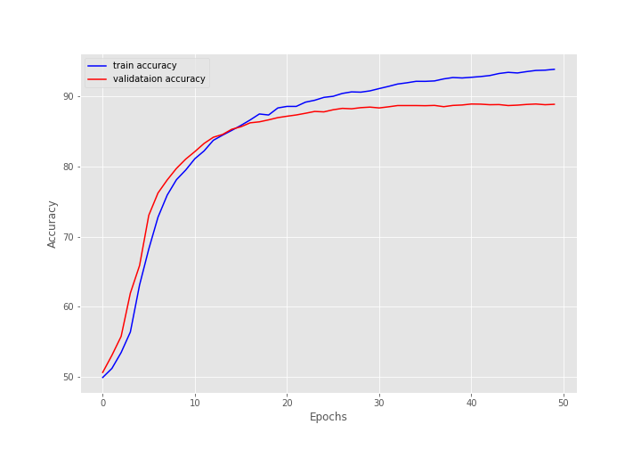
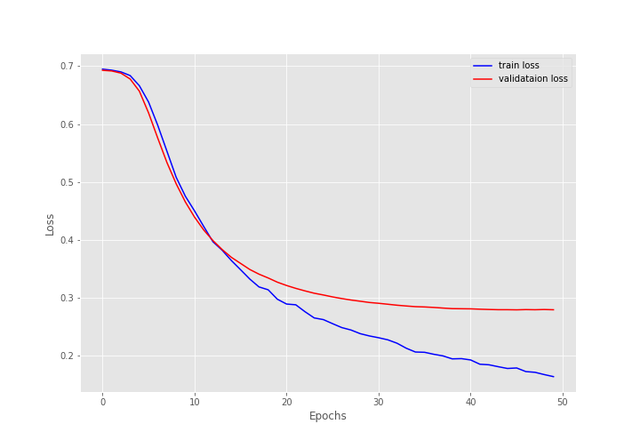
Both the accuracy and loss plots seem to be improving decently till the end of training. There is almost no fluctuation.

Testing the Trained IMDB Text Classification PyTorch Model

For testing the model, first, we will load the trained model from the disk.

trained_model = torch.load(
    os.path.join(OUTPUTS_DIR, 'model.pth')
)

Then we can call the validate function as the test data loader also contains the ground truth labels.

test_loss, test_acc = validate(
    trained_model, 
    test_loader,  
    criterion, 
    device
)

print(f"Test loss: {test_loss}, test acc: {test_acc}")

Here is the output.

Test loss: 0.28937702397910914, test acc: 87.88

The test accuracy is 87.88% which is very close to the validation accuracy. There is obviously scope to improve a lot here but this is good enough for starting out.

Inference on Unseen Reviews

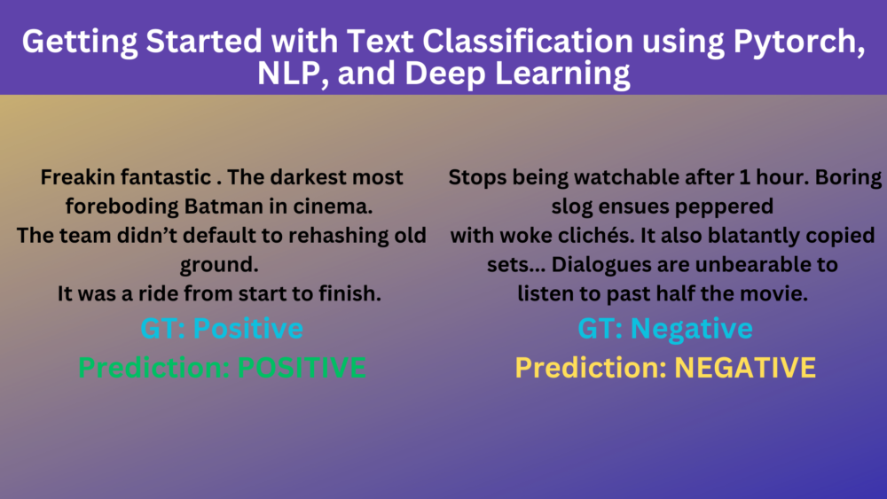
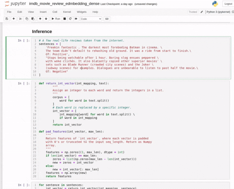
For the final part, we will run inference on unseen reviews. The reviews that we will use here have been taken from the Metacritic user reviews. So, they are just perfect to test our model. One of them is positive and the other is a negative review.

# A few real-life reviews taken from the internet.
sentences = [
    'Freakin fantastic . The darkest most foreboding Batman in cinema. \
    The team didn’t default to rehashing old ground. It was a ride from start to finish.',
    
    "Stops being watchable after 1 hour. Boring slog ensues peppered \
    with woke clichés. It also blatantly copied other superior movies' \
    sets such as Blade Runner (crowded city scenes) and the Joker \
    (subway scenes) for examples. Dialogues are unbearable to listen to past half the movie."
]

We again define two functions to convert words to integers and pad the features. This is to ensure that we can run the inference part of the notebook independently whenever restarting the notebook.

def return_int_vector(int_mapping, text):
    """
    Assign an integer to each word and return the integers in a list.
    """
    corpus = [
        word for word in text.split()
    ] 
    # Each word is replaced by a specific integer.
    int_vector = [
        int_mapping[word] for word in text.split() \
        if word in int_mapping
    ]
    return int_vector

def pad_features(int_vector, max_len):
    """
    Return features of `int_vector`, where each vector is padded 
    with 0's or truncated to the input seq_length. Return as Numpy 
    array.
    """
    features = np.zeros((1, max_len), dtype = int)
    if len(int_vector) <= max_len:
        zeros = list(np.zeros(max_len - len(int_vector)))
        new = zeros + int_vector
    else:
        new = int_vector[: max_len]
    features = np.array(new)
    return features

Finally, we can loop over the sentences and run the inference.

for sentence in sentences:
    int_vector = return_int_vector(int_mapping, sentence)
    padded_features = pad_features(int_vector, int(longest_sentence_length))
    input_tensor = torch.tensor(padded_features, dtype=torch.int32)
    input_tensor = input_tensor.unsqueeze(0)
    output = model(input_tensor.to(device))
    preds = torch.sigmoid(output)
    print(sentence)
    if preds > 0.5:
        print('Prediction: POSITIVE')
    else:
        print('Prediction: NEGATIVE')
    print('\n')

We get the following output from the model.

Freakin fantastic . The darkest most foreboding Batman in cinema.     The team didn’t default to rehashing old ground. It was a ride from start to finish.
Prediction: POSITIVE


Stops being watchable after 1 hour. Boring slog ensues peppered     with woke clichés. It also blatantly copied other superior movies'     sets such as Blade Runner (crowded city scenes) and the Joker     (subway scenes) for examples. Dialogues are unbearable to listen to past half the movie.
Prediction: NEGATIVE

Our PyTorch text classification model trained on the IMDB movie review dataset is able to correctly predict the labels of the reviews. This is very good news considering we have a very simple model with just two layers and it was trained entirely from scratch.

Summary and Conclusion

In this article, we covered a code-first approach to text classification using NLP and PyTorch. Of course, we did not go into a lot of detail regarding the basics of NLP. But we covered each step in detail and the bare minimum preprocessing that one needs to do for NLP text classification. We also did not cover a lot of details regarding the model. We will get into all those details in future articles. I hope that this article was worth your time.

If you have any doubts, thoughts, or suggestions, please leave them in the comment section. I will surely address them.

You can contact me using the Contact section. You can also find me on LinkedIn, and Twitter.