Training UNet from Scratch using PyTorch

UNet was a turning point for deep learning based semantic segmentation and in a way, still is. At the time of publication, it solved a lot of problems. One of which was training good semantic segmentation models with smaller datasets. In most cases, we can train the vanilla UNet from scratch on a completely new dataset and still get good results. To this, we will be training a UNet model from scratch using PyTorch in this article.

Training from scratch is not a significant requirement nowadays in most cases, even for semantic segmentation models. Libraries like Torchvision already provide a host of pretrained models which we can easily fine tune and get exceptional results. But Torchvision and many other libraries do not a pretrained model for UNet in their collection. For this reason, it will be fun to train our own model on a simple dataset and check the results.

After going through this article, you will know:

• Exactly what kind of changes do you need to make to the original UNet while training from scratch to get the best results?
• What kind of data processing is needed for training UNet from scratch?
• And what kind of results we can expect when training UNet on a small dataset?

Let’s jump into the article without any further delay.

The UNet Architecture

We implemented the UNet model from scratch using PyTorch in the previous article. While implementing, we discussed the changes that we made to the architecture compared to the original UNet architecture.

Still, our model was very close to the original architecture. For implementation, the story ends there. But for training the model from scratch on a completely new dataset, we need to make a few more changes to the architecture.

This ensures that we get the best results according to the current research scenario in deep learning. UNet may be an old architecture but is still pretty deep. The original UNet model has 10 convolutional layers in the contracting path and 8 in the expanding path. This is excluding the final layer. The residual connections help to a certain extent only.

So, what more changes will we be making?

To get the best results that we can, we will be also adding Batch Normalization in the Double Convolution module. It further helps to mitigate the issue of the vanishing gradient problem through a deep network like UNet.

The above figure shows how our modified UNet will look like while training from scratch.

We also cover the architecture once more in the coding section.

The Penn-Fudan Dataset

We will use the Penn-Fudan Pedestrian dataset for training the UNet model from scratch. This dataset contains images for pedestrian detection and segmentation. It has a total of 170 images and 345 labeled persons.

The original dataset can be found on the official Penn-Fudan Database for Pedestrian Detection and Segmentation website.

But we do not need the bounding box information for this project. So, I prepared a different version of the Penn-Fudan dataset only for semantic segmentation with proper training/validation split.

You can find the version of Penn-Fudan dataset for semantic segmentation on Kaggle. This version of the dataset contains 146 images for training and 24 images for validation.

The Penn-Fudan Pedestrian Segmentation Masks

The segmentation masks in the Penn-Fudan Pedestrian dataset are grayscale images. In each mask, the background has a pixel value of 0. While each person is indicated by an incrementing pixel value. This means if there are two persons, the instance of the first person has a pixel value of 1 and the second person has a pixel value of 2.

But while writing the dataset preparation code, we will replace all pixels other than 0 with 255. This will make the mask of each person entirely white and the rest of the code will also become simpler.

Here are a few images and their corresponding segmentation masks from the dataset.

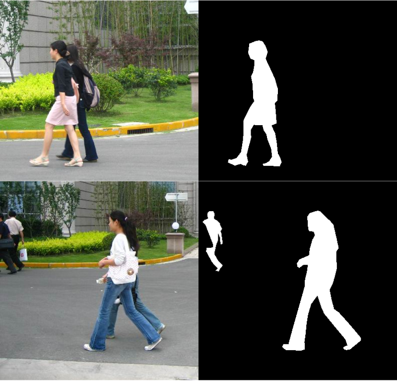
As you can see, the dataset is quite simple. This is just perfect for testing any semantic segmentation model training from scratch.

Training UNet from Scratch Project Directory Structure

Before moving further, let’s take a look at the project directory structure.

├── input
│   └── PennFudanPed
│       ├── train_images
│       ├── train_masks
│       ├── valid_images
│       └── valid_masks
├── outputs
│   ├── valid_preds [50 entries exceeds filelimit, not opening dir]
│   ├── accuracy.png
│   ├── best_model_iou.pth
│   ├── best_model_loss.pth
│   ├── loss.png
│   ├── miou.png
│   └── model.pth
└── src
    ├── config.py
    ├── datasets.py
    ├── engine.py
    ├── inference_image.py
    ├── metrics.py
    ├── model.py
    ├── train.py
    └── utils.py

• The input folder contains the Penn-Fudan Pedestrian dataset. The train_images & train_masks folders contain the training samples and the valid_images & valid_masks contain the corresponding validation samples.
• All the output files from training and validation go into the outputs directory.
• And the src directory contains the Python files. It contains 8 Python files. We will only go through the important sections of some of the necessary files.

All the code files along with the proper directory structure are available via a downloadable zip file that comes with the post. For training, you will need to download the Penn-Fudan Pedestrian segmentation dataset from Kaggle. If you wish to execute only the inference part, please find the weights files here.

PyTorch Version

The code in this project uses PyTorch 1.12.0 along with Albumentations for preprocessing of images and masks.

Please install them in case you plan on executing the code yourself.

Training UNet from Scratch on the Penn-Fudan Pedestrian Dataset

Let’s jump into the coding sections now. We have 8 Python files but will not visit all of them in detail. We will only go through the important parts of the code.

Download Code

The Configuration File

We have a config.py file in the src directory. It has the following contents.

ALL_CLASSES = ['background', 'person']

LABEL_COLORS_LIST = [
    (0, 0, 0), # Background.
    (255, 255, 255),
]

VIS_LABEL_MAP = [
    (0, 0, 0), # Background.
    (0, 255, 0),
]

It contains three lists.

• ALL_CLASSES holds the names of the classes in the dataset. We have a person class and a background class in the Penn-Fudan Pedestrian dataset.
• The LABEL_COLORS_LIST holds the pixel color mapping according to the ground truth masks. For the background class, all the pixels are 0. But in one of the earlier sections, we discussed that each pixel of a person has a value corresponding to its instance number. So, if there are two persons in one image, the pixel values for the first person will be 1 and for the second person 2. But we will take care of this while preparing the datasets and will change all the pixel values for person to 255.
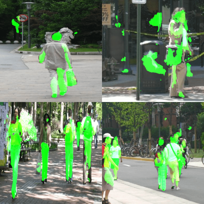
• The VIS_LABEL_MAP color mapping will be used for visualizations. Instead of white color, we will use green color for overlaying the segmentation results during inference.

That’s all there is to the config.py file.

Dataset Preparation

There are a few important points to handle while preparing the dataset. Let’s discuss them. All the dataset preparation code is present in the datasets.py file.

First of all, we need to make the pixel values containing a person 255. This is pretty easy and we can do it with just three lines of code.

# Make all instances of person 255 pixel value and background 0.
im = mask > 0
mask[im] = 255
mask[np.logical_not(im)] = 0

We make any pixel value greater than 0 equal to 255 for this dataset. You can find this code in the __getitem__ method of the SegmentationDataset class.

For normalization of the values, we are just dividing the image by 255.0. Note that we are doing this step only for the RGB images and not for the masks.

Next comes the augmentations. We are applying the following augmentations to prevent overfitting. Here, p indicates the probability value.

• HorizontalFlip (p=0.2)
• RandomBrightnessContrast (p=0.2)
• RandomSunFlare (p=0.2)
• RandomFog (p=0.2)
• Rotate (limit=25)

From experiments, I found that it is essential to apply extensive augmentations to prevent overfitting.

For the resizing, we will resize all the images and masks to 512×512 resolution while training. While this happens in the datasets.py file, we can easily control this using a command line flag for the train.py driver script. This allows more flexibility to train with desired image sizes.

The UNet Model

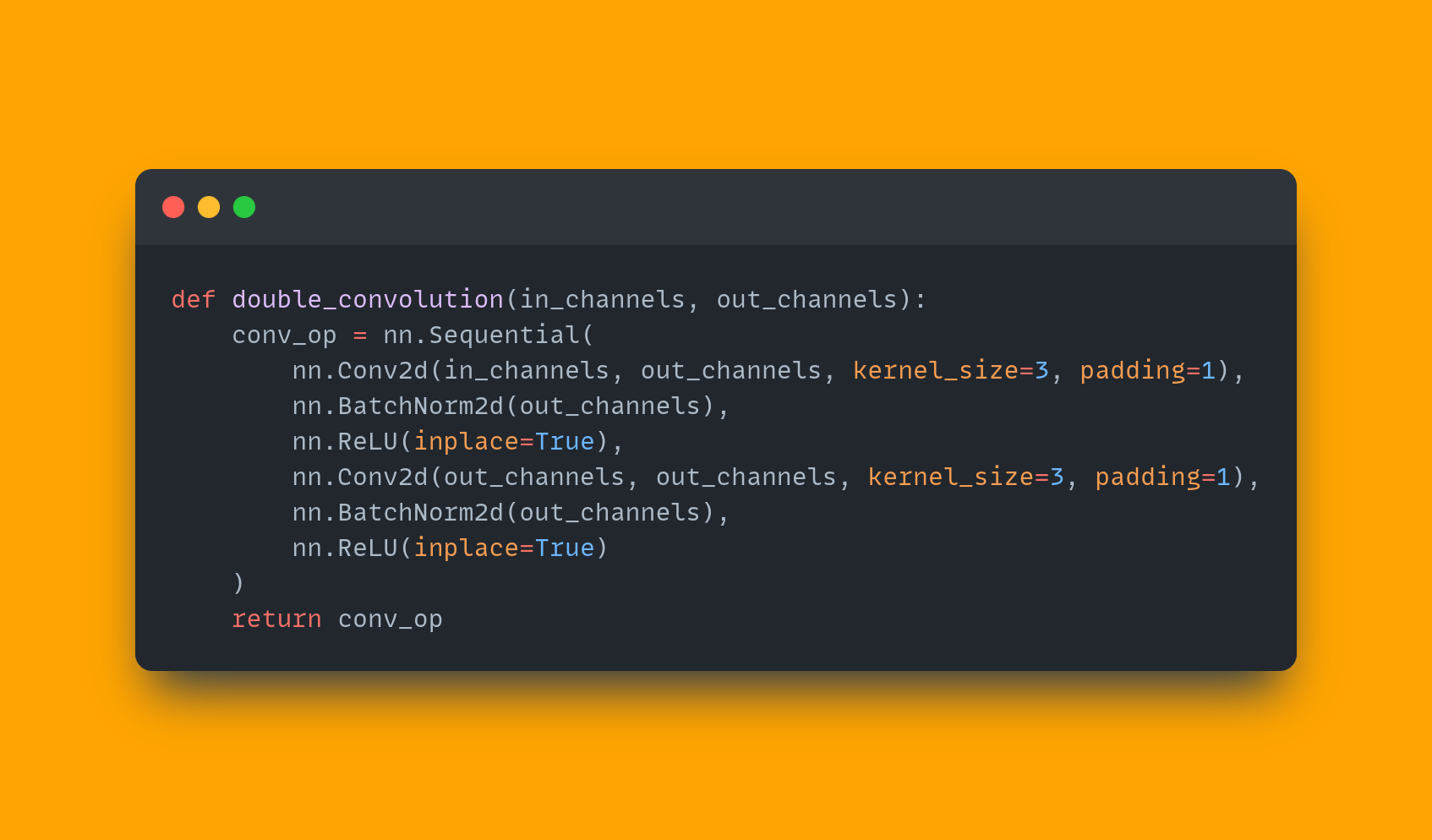
The UNet model remains almost the same as was in the previous post when implemented from scratch. The only thing new thing are the Batch Normalization layers in the double_convolution function.

For the sake of completion, the following block contains the entire UNet architecture.

import torch
import torch.nn as nn
import torch.nn.functional as F

def double_convolution(in_channels, out_channels):
    """
    In the original paper implementation, the convolution operations were
    not padded but we are padding them here. This is because, we need the 
    output result size to be same as input size.
    """
    conv_op = nn.Sequential(
        nn.Conv2d(in_channels, out_channels, kernel_size=3, padding=1),
        nn.BatchNorm2d(out_channels),
        nn.ReLU(inplace=True),
        nn.Conv2d(out_channels, out_channels, kernel_size=3, padding=1),
        nn.BatchNorm2d(out_channels),
        nn.ReLU(inplace=True)
    )
    return conv_op

class UNet(nn.Module):
    def __init__(self, num_classes):
        super(UNet, self).__init__()

        self.max_pool2d = nn.MaxPool2d(kernel_size=2, stride=2)

        # Contracting path.
        # Each convolution is applied twice.
        self.down_convolution_1 = double_convolution(3, 64)
        self.down_convolution_2 = double_convolution(64, 128)
        self.down_convolution_3 = double_convolution(128, 256)
        self.down_convolution_4 = double_convolution(256, 512)
        self.down_convolution_5 = double_convolution(512, 1024)

        # Expanding path.
        self.up_transpose_1 = nn.ConvTranspose2d(
            in_channels=1024, 
            out_channels=512,
            kernel_size=2, 
            stride=2)
        # Below, `in_channels` again becomes 1024 as we are concatinating.
        self.up_convolution_1 = double_convolution(1024, 512)
        self.up_transpose_2 = nn.ConvTranspose2d(
            in_channels=512, 
            out_channels=256,
            kernel_size=2, 
            stride=2)
        self.up_convolution_2 = double_convolution(512, 256)
        self.up_transpose_3 = nn.ConvTranspose2d(
            in_channels=256, 
            out_channels=128,
            kernel_size=2, 
            stride=2)
        self.up_convolution_3 = double_convolution(256, 128)
        self.up_transpose_4 = nn.ConvTranspose2d(
            in_channels=128, 
            out_channels=64,
            kernel_size=2, 
            stride=2)
        self.up_convolution_4 = double_convolution(128, 64)

        # output => increase the `out_channels` as per the number of classes.
        self.out = nn.Conv2d(
            in_channels=64, 
            out_channels=num_classes, 
            kernel_size=1
        ) 

    def forward(self, x):
        down_1 = self.down_convolution_1(x)
        down_2 = self.max_pool2d(down_1)
        down_3 = self.down_convolution_2(down_2)
        down_4 = self.max_pool2d(down_3)
        down_5 = self.down_convolution_3(down_4)
        down_6 = self.max_pool2d(down_5)
        down_7 = self.down_convolution_4(down_6)
        down_8 = self.max_pool2d(down_7)
        down_9 = self.down_convolution_5(down_8)        
        # *** DO NOT APPLY MAX POOL TO down_9 ***
        
        up_1 = self.up_transpose_1(down_9)
        x = self.up_convolution_1(torch.cat([down_7, up_1], 1))

        up_2 = self.up_transpose_2(x)
        x = self.up_convolution_2(torch.cat([down_5, up_2], 1))

        up_3 = self.up_transpose_3(x)
        x = self.up_convolution_3(torch.cat([down_3, up_3], 1))

        up_4 = self.up_transpose_4(x)
        x = self.up_convolution_4(torch.cat([down_1, up_4], 1))

        out = self.out(x)
        return out

As you can see, we have the BatchNorm2d layers after the Conv2d layers in the double_convolution function. This is the only change that we make to the model architecture.

Training the UNet Model

We have almost all the essential things in place and can move on to training the UNet model from scratch.

We have left out the discussion of some of the code files. But feel free to go through them before getting into the training part.

We will use the train.py script to train the UNet model. This file supports a few command line flags. Let’s check them out.

• --epochs: The number of epochs that we want to train the UNet model for.
• --lr: The initial learning rate for the optimizer.
• --batch: Batch size for the data loader.
• --imgsz: Image resize resolution. If we pass 512, then the final resolution will be 512×512. The default value is 512.
• --scheduler: It is a boolean flag. If we pass this, then the learning rate will reduce by a factor of 10 after 60 epochs.

All the training and inference experiments were conducted on a machine with 10 GB RTX 3080 GPU, 10th generation i7 CPU, and 32 GB RAM. If you wish to run inference only, please download the trained weights from here.

You can execute the following command in a terminal within the src directory to start the training.

python train.py --epochs 125 --batch 4 --lr 0.005

We are training the UNet model for 125 epochs with a batch size of 4 and a learning rate of 0.005. As we are training from scratch, the learning rate is a bit higher.

Here are the truncated outputs.

Namespace(epochs=125, lr=0.005, batch=4, imgsz=512, scheduler=False)
UNet(
  (max_pool2d): MaxPool2d(kernel_size=2, stride=2, padding=0, dilation=1, ceil_mode=False)
  (down_convolution_1): Sequential(
    (0): Conv2d(3, 64, kernel_size=(3, 3), stride=(1, 1), padding=(1, 1))
    (1): BatchNorm2d(64, eps=1e-05, momentum=0.1, affine=True, track_running_stats=True)
    (2): ReLU(inplace=True)
    (3): Conv2d(64, 64, kernel_size=(3, 3), stride=(1, 1), padding=(1, 1))
    (4): BatchNorm2d(64, eps=1e-05, momentum=0.1, affine=True, track_running_stats=True)
    (5): ReLU(inplace=True)
  )
.
.
.
31,043,586 total parameters.
31,043,586 training parameters.
Adjusting learning rate of group 0 to 5.0000e-03.
EPOCH: 1
Training
|                    | 37/? [00:17<00:00,  2.06it/s]                                                                                                                                          
Validating
100%|████████████████████| 6/6 [00:01<00:00,  5.87it/s]                                                                                                                                       

Best validation loss: 0.4590298682451248

Saving best model for epoch: 1


Best validation IoU: 0.35901248600848085

Saving best model for epoch: 1

Train Epoch Loss: 0.5186, Train Epoch PixAcc: 0.7824, Train Epoch mIOU: 0.455493
Valid Epoch Loss: 0.4590, Valid Epoch PixAcc: 0.7138 Valid Epoch mIOU: 0.359012
--------------------------------------------------
.
.
.
EPOCH: 120
Training
|                    | 37/? [00:13<00:00,  2.74it/s]                                                                                                                                          
Validating
100%|████████████████████| 6/6 [00:01<00:00,  5.74it/s]                                                                                                                                       

Best validation IoU: 0.6838485418037938

Saving best model for epoch: 120

Train Epoch Loss: 0.1836, Train Epoch PixAcc: 0.9006, Train Epoch mIOU: 0.755486
Valid Epoch Loss: 0.1729, Valid Epoch PixAcc: 0.7979 Valid Epoch mIOU: 0.683849
--------------------------------------------------
.
.
.
--------------------------------------------------
EPOCH: 125
Training
|                    | 37/? [00:14<00:00,  2.64it/s]                                                                                                                                          
Validating
100%|████████████████████| 6/6 [00:01<00:00,  5.61it/s]                                                                                                                                       
Train Epoch Loss: 0.1681, Train Epoch PixAcc: 0.9076, Train Epoch mIOU: 0.773854
Valid Epoch Loss: 0.1679, Valid Epoch PixAcc: 0.7991 Valid Epoch mIOU: 0.682702
--------------------------------------------------
TRAINING COMPLETE

We are saving two models, one according to the best validation loss (least loss) and another according to the highest mean IoU value.

For, the above training run, the best model for mean IoU got saved on epoch 120. We achieve the best mean IoU of 68.38.

Analyzing the Graphs

The following are the loss, accuracy, and mean IoU graphs.

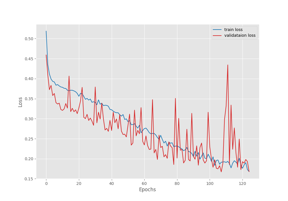
Even though the validation loss graph seems to fluctuate, it is following a decreasing trend till the end of training.

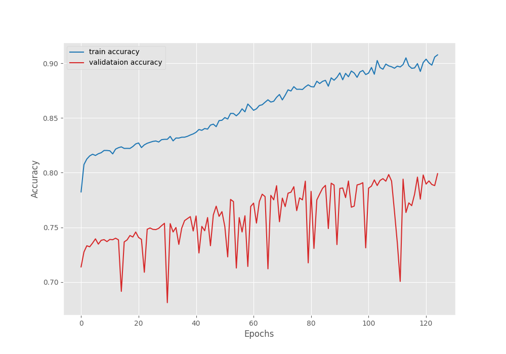
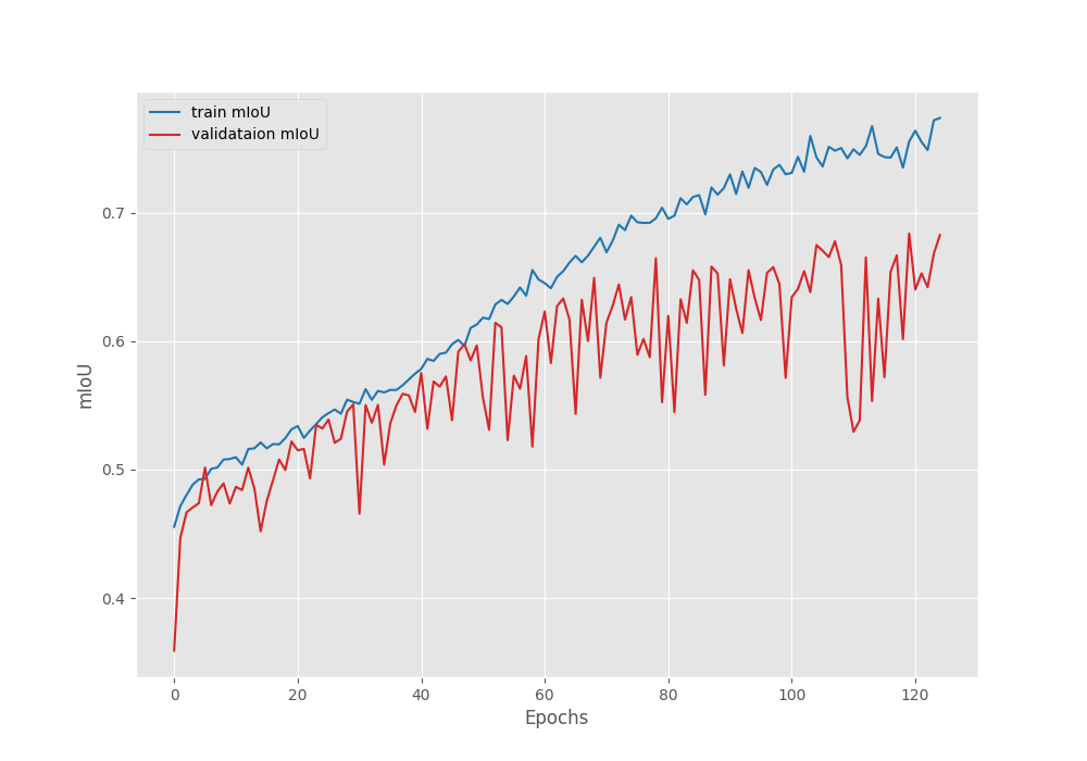
The plots for the validation accuracy and mean IoU also follow a similar trend. They both almost keep on improving till the end.

We do not see long plateaus or constant deterioration of the validation plots. And most probably this is possible due to the extreme augmentations that we apply to the training images.

Inference using the Trained UNet Model

We have the trained UNet model with us. Also, we have the validation images from the Penn-Fudan Pedestrian dataset. Although they were already used in the validation loop while training the model, we can still use them for inference.

We can run inference on images in a directory using the inference_image.py script.

python inference_image.py --model ../outputs/best_model_iou.pth --input ../input/PennFudanPed/valid_images/ --imgsz 512

We provide the path to the best mean IoU model using --models flag. The --input flag accepts the path to a directory containing images. And --imgsz is the image resizing factor. We resize the images to 512×512 resolution during inference which is the same as was for training.

All the results will be saved inside the outputs/inference_results directory.

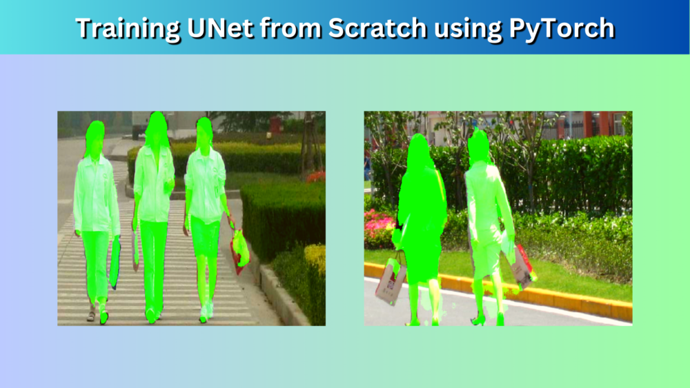
Here are a few results where the model performed well, if not the best.

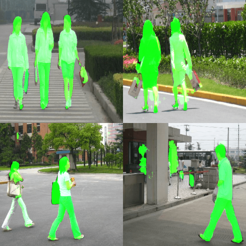
We can see that the model performs well but not very well obviously. In some cases, it is able to differentiate between a person and a handbag, while in some other cases, it isn’t. For sure, there is scope for improvement.

Here are some other images, where the model performed considerably worse.

In the above cases, the model is not able to segment the persons properly at all.

It looks like, the model may need even more training with data augmentation and then it will be able to perform well. Also, we had only 146 samples for training. Having more training instances will surely help the model.

Articles on Semantic Segmentation You Should Not Miss

Here is a list of a few articles on semantic segmentation in case you want to dive deeper into the topic.

• Semantic Segmentation using PyTorch DeepLabV3 and Lite R-ASPP with MobileNetV3 Backbone
• YOLOP for Panoptic Driving Perception
• YOLOP ONNX Inference on CPU
• Inference Using YOLOPv2 PyTorch

Summary and Conclusion

In this article, we tried training a UNet semantic segmentation from scratch on the Penn-Fudan Pedestrian segmentation dataset. After training, we also carried out inference on the validation images. The results were not the best, but also not very bad for training from scratch with only 146 samples. The next step for this project will be to try out some data augmentation, and see whether we can prevent overfitting and train a better model.

I hope that this article was helpful to you.

If you have any doubts, thoughts, or suggestions, please leave them in the comment section. I will surely address them.

You can contact me using the Contact section. You can also find me on LinkedIn, and Twitter.

References

• Penn-Fudan Pedestrian dataset