Implementing UNet from Scratch Using PyTorch

When implementing a semantic segmentation project, we use pretrained models from libraries like Torchvision. But sometimes, implementing a few semantic segmentation architectures from scratch is better. One of the reasons may be that the pretrained model is not available in many of the vision libraries. Or, by implementing a model from scratch, we understand its architecture thoroughly. In this article, we will implement the UNet model from scratch using PyTorch.

UNet is a famous architecture that is still relevant to date. It’s not very complicated to implement from scratch as well. There are a few intricacies of course which we will cover while implementing the architecture.

We will cover the following points in this article:

• We will start with the discussion of the UNet architecture from the paper.
• While discussing the architecture, we will note which parts of the architecture we will exactly follow and which parts we will make small changes to. We will adhere to some modern and better choices of deep learning architecture which were not implemented into the original UNet model.
• Then we will get into the coding section. This is where we will start implementing the UNet model from scratch using PyTorch.
• After the implementation, we will do a small sanity check to ensure that the model is correct.

Note: We will not be training the UNet model in this post. We will just implement it from scratch. We will train this exact model in the next article.

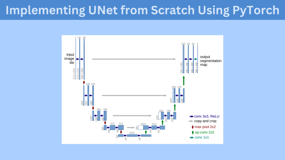
The UNet Model Architecture

The UNet model was introduced in the paper “U-Net: Convolutional Networks for Biomedical
Image Segmentation” by Olaf Ronneberger, Philipp Fischer, and Thomas Brox.

The authors wanted to create UNet for medical imaging training. Most of the time, in medical imaging, we do not have sufficient samples to train. Previous semantic segmentation architectures did not perform very well when trained on insufficient medical imaging samples. For their experiments, the authors chose the HeLa cells dataset.

The main aim of the authors was to create a semantic segmentation model that could overcome the large dataset requirement for training. According to them, it was possible by:

• Making better architecture choices while building the deep learning model.
• And using good augmentation techniques on the dataset while training the model.

This led to the creation of the UNet model for semantic segmentation.

We will not focus much on the dataset augmentation part in this article. As we are implementing UNet from scratch using PyTorch, we will focus entirely on the model architecture.

UNet Architecture Details

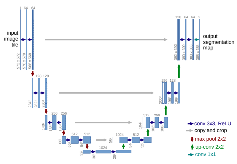
The above figure shows the UNet architecture. And it is quite apparent why it is called UNet. We can see that it has a U-shape with two paths.

The path on the left side is the contracting path and the path on right is the expanding path.

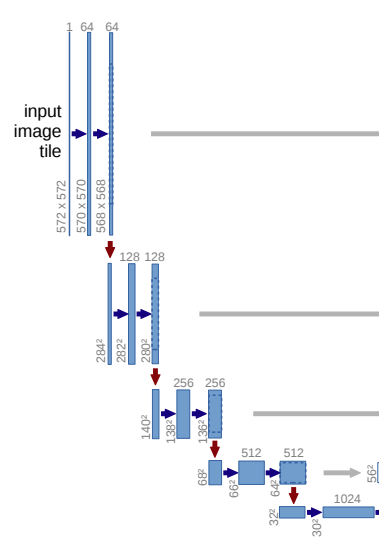
The contracting path reduces the size of the feature maps starting from the original image.

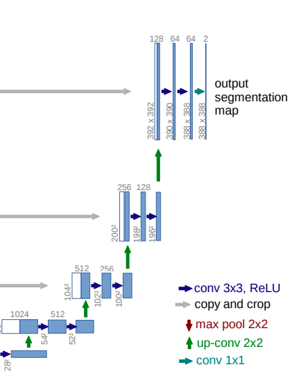
Similarly, the expanding path keeps on expanding the size of the feature maps till we reach the last layer.

The grey arrows between the contracting and expanding show the skip connections. We concatenate the feature maps from the corresponding contracting and expanding path. This is very similar to the Residual connections in ResNets. This allows the model to remember the features from past layers and reduces the chances of vanishing gradient when the network is too deep.

Please, do note that we concatenate the features along the channel axis. Also, the original UNet crops and concatenates the features from the contracting path to the expanding path. According to the authors, cropping is necessary due to the loss of border pixels in every convolution.

There is another important point to notice in the above image. The input to the UNet model is an image with a spatial resolution of 572×572. But the output has a spatial resolution of 388×388. This is because the original UNet model does not use any padding during convolutions.

How Our UNet from Scratch using PyTorch Differ Compared to the Original One?

This brings us to the next important discussion. How our implementation of UNet from scratch using PyTorch will differ from the original one:

• Firstly, we will not take cropping into consideration while concatenating the feature maps from contracting and expanding paths.
• Secondly, we will use padding in the contracting path. This will make the output feature map the same size as the input image. This is important because most of the modern semantic segmentation architectures follow this rule.

The above covers most of the details that we need to know about UNet architecture. There are a few more details that we will discuss while writing the UNet code from scratch using PyTorch.

Implementing UNet from Scratch using PyTorch

Let’s get down to the implementation of the UNet model from scratch using PyTorch without any further delay.

We just have one Python file for this project, that is, unet.py. All the code will reside inside this one file.

While implementing, we will break the entire code into three subsections. They are:

• The Double Convolution function.
• The UNet model class.
• And the main block (for sanity check).

Implementing Double Convolution Function for UNet.

If we take a closer look at the model architecture, we can find that there are always two consecutive convolutional blocks.

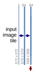
For example, after the input image tile, we have two 3×3 2D convolutions with followed by ReLU.

Similarly, after every 2D Max Pooling layer, we have two 2D convolutional layers. You can see the downward red arrow followed by two blue arrows in the contracting path of the UNet.

This is even true for the expanding path. Here, we have the up-convolution (green arrow). Following this are two blue arrows representing the two 2D convolutional layers.

So, instead of writing these consecutive convolutional manually each time, we can put them in a function and call them.

Download Code

The following code block contains the import statements and the double_convolution function.

import torch
import torch.nn as nn

def double_convolution(in_channels, out_channels):
    """
    In the original paper implementation, the convolution operations were
    not padded but we are padding them here. This is because, we need the 
    output result size to be same as input size.
    """
    conv_op = nn.Sequential(
        nn.Conv2d(in_channels, out_channels, kernel_size=3, padding=1),
        nn.ReLU(inplace=True),
        nn.Conv2d(out_channels, out_channels, kernel_size=3, padding=1),
        nn.ReLU(inplace=True)
    )
    return conv_op

We build a Sequential block with two Conv2d layers followed by ReLU activation.

There is another important point to notice here. We are using a padding of 1 for each of the convolutional layers. We will use this double_convolution function during the building of the contracting and expanding path. So, the padding will ensure that the final segmentation map is the same size as the input image.

The UNet Model Class

Next, we have the UNet model class. The code block here is going to be a bit long. But let’s write it completely once to avoid confusion.

class UNet(nn.Module):
    def __init__(self, num_classes):
        super(UNet, self).__init__()

        self.max_pool2d = nn.MaxPool2d(kernel_size=2, stride=2)

        # Contracting path.
        # Each convolution is applied twice.
        self.down_convolution_1 = double_convolution(3, 64)
        self.down_convolution_2 = double_convolution(64, 128)
        self.down_convolution_3 = double_convolution(128, 256)
        self.down_convolution_4 = double_convolution(256, 512)
        self.down_convolution_5 = double_convolution(512, 1024)

        # Expanding path.
        self.up_transpose_1 = nn.ConvTranspose2d(
            in_channels=1024, out_channels=512,
            kernel_size=2, 
            stride=2)
        # Below, `in_channels` again becomes 1024 as we are concatinating.
        self.up_convolution_1 = double_convolution(1024, 512)
        self.up_transpose_2 = nn.ConvTranspose2d(
            in_channels=512, out_channels=256,
            kernel_size=2, 
            stride=2)
        self.up_convolution_2 = double_convolution(512, 256)
        self.up_transpose_3 = nn.ConvTranspose2d(
            in_channels=256, out_channels=128,
            kernel_size=2, 
            stride=2)
        self.up_convolution_3 = double_convolution(256, 128)
        self.up_transpose_4 = nn.ConvTranspose2d(
            in_channels=128, out_channels=64,
            kernel_size=2, 
            stride=2)
        self.up_convolution_4 = double_convolution(128, 64)

        # output => `out_channels` as per the number of classes.
        self.out = nn.Conv2d(
            in_channels=64, out_channels=num_classes, 
            kernel_size=1
        ) 

    def forward(self, x):
        down_1 = self.down_convolution_1(x)
        down_2 = self.max_pool2d(down_1)
        down_3 = self.down_convolution_2(down_2)
        down_4 = self.max_pool2d(down_3)
        down_5 = self.down_convolution_3(down_4)
        down_6 = self.max_pool2d(down_5)
        down_7 = self.down_convolution_4(down_6)
        down_8 = self.max_pool2d(down_7)
        down_9 = self.down_convolution_5(down_8)        
        # *** DO NOT APPLY MAX POOL TO down_9 ***
        
        up_1 = self.up_transpose_1(down_9)
        x = self.up_convolution_1(torch.cat([down_7, up_1], 1))

        up_2 = self.up_transpose_2(x)
        x = self.up_convolution_2(torch.cat([down_5, up_2], 1))

        up_3 = self.up_transpose_3(x)
        x = self.up_convolution_3(torch.cat([down_3, up_3], 1))

        up_4 = self.up_transpose_4(x)
        x = self.up_convolution_4(torch.cat([down_1, up_4], 1))

        out = self.out(x)
        return out

The __init__() Method

Let’s start with the __init__() method.

We define a MaxPool2d layer first. We will use this after every downsampling module.

From lines 9 to 13, we define the contracting path. Each time, we call the double_convolution function with the necessary number of in_channels and out_channels. If you take a look at the diagram, this is exactly the same as paper. We start from a out_channels of 64 in the first layer and finish with 1024 out_channels just before the expanding path begins.

Starting from line 16, we have the layer definitions for the expanding path. We use 2D Transposed Convolutional layers for this. The very first layer of expanding path reduces the output channels from 1024 to 512. Then we have the rest of the layer definitions for double_convolution and transposed convolution.

There is a very important point to note here. Each of the double_convolution definitions in the expanding path has twice the number of in_channels as the number of out_channels in the previous transposed convolution. Why is that? This is because of the skip connections. The skip connections between the contracting and expanding path will happen along the channel axis. So, before the double convolutions, the number of input channels will double.

The forward() Method

The forward method simply contains the stacking of all the layers in the proper order. A double convolution block follows each of the transposed convolutional layers.

Starting with the contracting path. We have alternate downsampling and max-pooling from lines 45 to 53. Following the original UNet architecture, we do not apply max-pooling after the final downsampling block. This is where the output channels are 1024.

Starting from line 56 we have the expanding path layers. The double convolutions follow transposed convolutions layers. Also, notice that the concatenation happens in reverse order. Meaning, the first transposed convolutional layer concatenates along the channel axis with the last downsampled block, and so on.

The very final layer has the output channels same as the number of classes in the dataset. Also, the final layer is a 2D convolution as it is a segmentation architecture and we need the final feature map. To avoid reduction in spatial resolution, almost always, the final layer will have a kernel size of 1.

A Sanity Check Through Forward Pass

We can do a simple forward pass inside the main block to check that the input image size and the output feature map size match up.

if __name__ == '__main__':
    input_image = torch.rand((1, 3, 512, 512))
    model = UNet(num_classes=10)
    # Total parameters and trainable parameters.
    total_params = sum(p.numel() for p in model.parameters())
    print(f"{total_params:,} total parameters.")
    total_trainable_params = sum(
        p.numel() for p in model.parameters() if p.requires_grad)
    print(f"{total_trainable_params:,} training parameters.")
    outputs = model(input_image)
    print(outputs.shape)

We can execute the file using the following command.

python unet.py

Following is the output.

31,032,330 total parameters.
31,032,330 training parameters.
torch.Size([1, 10, 512, 512])

There are around 31 million parameters in the model. Also, the final feature map size matches the input image size of 512×512. So, it looks like our model is working as expected.

This is all about implementing UNet from scratch using PyTorch.

Articles on Semantic Segmentation You Should Not Miss

Here is a list of a few articles on semantic segmentation in case you want to dive deeper into the topic.

• Semantic Segmentation using PyTorch FCN ResNet50
• Semantic Segmentation using PyTorch DeepLabV3 and Lite R-ASPP with MobileNetV3 Backbone
• YOLOP for Panoptic Driving Perception
• YOLOP ONNX Inference on CPU
• Inference Using YOLOPv2 PyTorch

Summary and Conclusion

In this article, we implemented the UNet semantic segmentation model from scratch using PyTorch. First, we went through the architecture introduced in the paper. Then we discussed how our implementation will differ in a few ways. And finally, we implemented the architecture. I hope that this article was useful to you.

If you have any doubts, thoughts, or suggestions, please leave them in the comment section. I will surely address them.

You can contact me using the Contact section. You can also find me on LinkedIn, and Twitter.