Early Apple Scab Recognition using Deep Learning

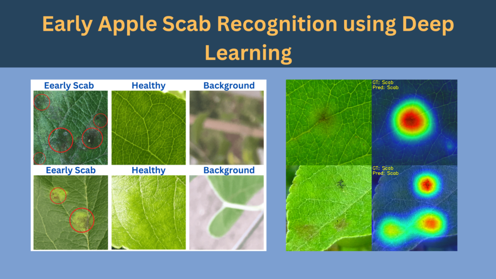
In this tutorial, we will train a deep neural network model for the recognition of early apple scab disease.

Deep learning for plant pathology is an active area of research. In fact, it is quite evident that in a few years, deep learning will help the field of agriculture and plantation to a great extent.

Starting from this post, we will be covering a series of 3 tutorials. All of them will be focused on detecting scab diseases in apple plants. Two of them will be image classification problems and one object detection problem. All of them will revolve around similar types of datasets (recognizing scab disease in apple plants). Such a series will surely give us a proper idea of how well deep learning and computer vision are capable of solving plant pathology.

We will cover the following points in this tutorial:

• First, we will start with the exploration of the Early Apple Scab Disease dataset.
• Secondly, we will discuss the code structure of the tutorial.
• Then we will move on to the coding part of the tutorial. Here, we will discuss the deep learning model to use for training, the data augmentation techniques, and the hyperparameters to use for training.
• After training the model, we will run it through an unseen test set to measure its accuracy.
• Along with that, we will also visualize the class activation maps of the test images. This will show us what part of the image the model focuses on while making the predictions.

Let’s start the journey of early apple scab recognition using deep learning.

Early Apple Scab Disease

Scab is a common fungal disease in apple plants. It can either affect the leaves or the fruits. Sometimes, it can become so severe that the fruits become inedible.

In this tutorial, we will focus on recognizing scab disease in apple leaves with early onset. Researchers try to differentiate between the early and advanced stages of apple scabs in the leaves on a regular basis. But deep learning techniques which have been trained on the advanced stages of apple scab disease images are unable to recognize the early stages of apple scab. For this reason, it is often a requirement to train a CNN-based image classification model in the early stages of the apple scab disease as well.

The eAppleScab Dataset

In this tutorial, we will use the eAppleScab dataset from Kaggle. The dataset contains images of apple leaves that have been infected by scab disease in the early stage. The dataset also has an accompanying paper.

The images in the dataset are 525×525 pixels in size. All are RGB images and have been classified into three classes:

• Background: Images that do not contain any healthy leaves or leaves affected by scab disease.
• Healthy: Images of leaves that are not affected by scab disease.
• Scab: Leaves with scab disease.

The Background, Healthy, and Scab classes contain 703, 768, and 700 images respectively. All of them are in their respective folders. Later on, we will sample out a few images for testing which will not be part of either the training or validation set.

The red circles in figure 2 point to the early scab disease on the apple leaves. It is quite evident that early recognition of scab disease can sometimes be difficult. Because many cases, the affected region may have only subtle indications of the disease.

Humans may find it difficult to recognize such early stages of apple scab by the naked eye. But as we will see later on, a convolutional neural network is quite capable to do so.

For now, you may download the dataset. In the next section, we will see how to structure the dataset in the project directory after extracting it.

Directory Structure

Let’s take a look at the directory structure for the project.

├── input
│   ├── eScab
│   │   ├── Background
│   │   ├── Healthy
│   │   └── Scab
│   ├── test
│       ├── Background
│       ├── Healthy
│       └── Scab
├── outputs
│   ├── cam_results [192 entries exceeds filelimit, not opening dir]
│   ├── test_results [192 entries exceeds filelimit, not opening dir]
│   ├── accuracy.png
│   ├── best_model.pth
│   ├── loss.png
│   └── model.pth
└── src
    ├── cam.py
    ├── datasets.py
    ├── model.py
    ├── prepare_test_data.py
    ├── test.py
    ├── train.py
    └── utils.py

• The input folder contains the dataset in the eScab subfolder. Each of the folders with the class names holds the corresponding images. We also have a test folder that contains 64 images from each class randomly sampled to be used for testing after training the model.
• The outputs directory contains all the outputs that we obtain during the training and testing of the model.
• And the src directory contains 7 Python code files. During the discussion of the coding part, we will go into the details of the code files.

Downloading the zip file for this post will give you access to all the code files along with the above directory structure. You will just need to download the dataset and prepare it in the structure shown above.

The PyTorch Version

The code uses PyTorch 1.12.0 along with Torchvision 0.13.0. As we are using the latest API for pretrained models in this post, you will at least need PyTorch 1.12.0.

You can find the installation commands for PyTorch 1.12.0 version at this link.

Visit the installation home page to install the latest version of PyTorch.

Early Apple Scab Recognition using Deep Learning and PyTorch

Let’s get into the practical part of this tutorial now. We will get into the technical details in each of the following subsections.

First, we will prepare the test set from the original dataset that we get from Kaggle.

Randomly Sampling Images for Testing

We will sample 64 images from each class of the original dataset for testing. This, we will use as a held-out set for testing the model after the training is complete.

Download Code

The prepare_test_data.py contains the entire code for this.

"""
Script to move a few images from the the original dataset
into the test dataset folder randomly.
"""

import shutil
import glob
import random
import os

random.seed(42)

ROOT_DIR = os.path.join('..', 'input', 'eScab')
DEST_DIR = os.path.join('..', 'input', 'test')
# Class directories.
class_dirs = ['Background', 'Healthy', 'Scab']
# Test images.
test_image_num = 64

for class_dir in class_dirs:
    os.makedirs(os.path.join(DEST_DIR, class_dir), exist_ok=True)
    init_image_paths = glob.glob(os.path.join(ROOT_DIR, class_dir, '*'))
    print(f"Initial number of images for class {class_dir}: {len(init_image_paths)}")
    random.shuffle(init_image_paths)
    for i in range(test_image_num):
        image_name = init_image_paths[i].split(os.path.sep)[-1]
        shutil.move(
            init_image_paths[i], 
            os.path.join(DEST_DIR, class_dir, image_name)
        )
    final_image_paths = glob.glob(os.path.join(ROOT_DIR, class_dir, '*'))
    print(f"Final number of images for class {class_dir}: {len(final_image_paths)}\n")

As you can see, we are moving 64 images from the original folder into the test folder under each of the class name subfolders. This reduces the number of images from the original eScab directory. In case you want all the original images back, you can just extract the original zip file that was downloaded from Kaggle.

To execute the script, run the following command within the src directory.

python prepare_test_data.py

You should see the following output on the terminal.

Initial number of images for class Background: 703
Final number of images for class Background: 639

Initial number of images for class Healthy: 768
Final number of images for class Healthy: 704

Initial number of images for class Scab: 700
Final number of images for class Scab: 636

This was the only manual dataset preparation step for the project. Now, we can move ahead into the deep learning part for early apple scab recognition.

Utilities and Helper Functions for Early Apple Scab Recognition

We will need a set of utilities and helper functions as we train the model. These include:

• Saving the best model according to the lowest validation loss.
• Saving the model after every epoch.
• Plotting the loss and accuracy graphs.

The utils.py file takes care of this.

import torch
import matplotlib
import matplotlib.pyplot as plt
import os

matplotlib.style.use('ggplot')

class SaveBestModel:
    """
    Class to save the best model while training. If the current epoch's 
    validation loss is less than the previous least less, then save the
    model state.
    """
    def __init__(
        self, best_valid_loss=float('inf')
    ):
        self.best_valid_loss = best_valid_loss
        
    def __call__(
        self, current_valid_loss, epoch, model
    ):
        if current_valid_loss < self.best_valid_loss:
            self.best_valid_loss = current_valid_loss
            print(f"\nBest validation loss: {self.best_valid_loss}")
            print(f"\nSaving best model for epoch: {epoch+1}\n")
            torch.save({
                'epoch': epoch+1,
                'model_state_dict': model.state_dict(),
                }, os.path.join('..', 'outputs', 'best_model.pth'))

The SaveBestModel class saves the model state dictionary and epoch number if the current epoch’s validation loss is lower than the previous lowest loss.

def save_model(epochs, model, optimizer, criterion):
    """
    Function to save the trained model to disk.
    """
    torch.save({
                'epoch': epochs,
                'model_state_dict': model.state_dict(),
                'optimizer_state_dict': optimizer.state_dict(),
                'loss': criterion,
                }, os.path.join('..', 'outputs', 'model.pth'))

The above code block contains the save_model function. It saves the model state dictionary, the number of epochs trained for, the optimizer state, and also the loss information after the training is complete. In case we need it, we can use it to resume training also.

def save_plots(train_acc, valid_acc, train_loss, valid_loss):
    """
    Function to save the loss and accuracy plots to disk.
    """
    # Accuracy plots.
    plt.figure(figsize=(10, 7))
    plt.plot(
        train_acc, color='tab:blue', linestyle='-', 
        label='train accuracy'
    )
    plt.plot(
        valid_acc, color='tab:red', linestyle='-', 
        label='validataion accuracy'
    )
    plt.xlabel('Epochs')
    plt.ylabel('Accuracy')
    plt.legend()
    plt.savefig(os.path.join('..', 'outputs', 'accuracy.png'))
    
    # Loss plots.
    plt.figure(figsize=(10, 7))
    plt.plot(
        train_loss, color='tab:blue', linestyle='-', 
        label='train loss'
    )
    plt.plot(
        valid_loss, color='tab:red', linestyle='-', 
        label='validataion loss'
    )
    plt.xlabel('Epochs')
    plt.ylabel('Loss')
    plt.legend()
    plt.savefig(os.path.join('..', 'outputs', 'loss.png'))

Finally, the save_plots function will save the loss and accuracy graphs in the outputs folder after the training.

Preparing the Early Apple Scab Recognition Dataset

The preparation of the datasets and data loaders will be quite simple.

Let’s start with initializing some constants and defining the training and validation transforms. All the dataset preparation code will go into the datasets.py file.

import os
import torch

from torchvision import datasets, transforms
from torch.utils.data import DataLoader, Subset

# Required constants.
ROOT_DIR = os.path.join('..', 'input', 'eScab')
IMAGE_SIZE = 512 # Image size of resize when applying transforms.
BATCH_SIZE = 16
NUM_WORKERS = 4 # Number of parallel processes for data preparation.
VALID_SPLIT = 0.15 # Ratio of data for validation

# Training transforms
def get_train_transform(image_size):
    train_transform = transforms.Compose([
        transforms.Resize((image_size, image_size)),
        transforms.RandomHorizontalFlip(p=0.5),
        transforms.RandomVerticalFlip(p=0.5),
        transforms.RandomRotation(35),
        transforms.ColorJitter(brightness=0.4,
                               contrast=0.4,
                               saturation=0.4,
                               hue=0),
        transforms.GaussianBlur(kernel_size=3, sigma=(0.5, 1.5)),
        transforms.RandomAdjustSharpness(sharpness_factor=2, p=0.5),
        transforms.ToTensor(),
        transforms.Normalize(
            mean=[0.485, 0.456, 0.406],
            std=[0.229, 0.224, 0.225]
            )
    ])
    return train_transform

# Validation transforms
def get_valid_transform(image_size):
    valid_transform = transforms.Compose([
        transforms.Resize((image_size, image_size)),
        transforms.ToTensor(),
        transforms.Normalize(
            mean=[0.485, 0.456, 0.406],
            std=[0.229, 0.224, 0.225]
            )
    ])
    return valid_transform 

We are defining the following as part of the constants:

• Path to the root dataset directory.
• Image size, which is 512×512 pixels in this case. You may notice that is higher than the regular image classification image sizes that generally go for 224×224 pixels. The reason for this is that the early scab disease may not be visible after resizing an image to around 200×200 pixels. Also, from experiments, it was clear that higher-resolution images tend to perform better.
• We are using a batch size of 16 with 4 parallel workers.
• We are using 15% of the data for validation and the rest for training.

The get_train_transform function has quite a few augmentations along with converting the images to tensor and normalizing them. All these augmentations help prevent overfitting and also allow the model to be trained longer. Along with that, it helps the model to learn to classify the scab disease under various lighting, color, and sharpness conditions.

The following figure shows what the augmented images may look like.

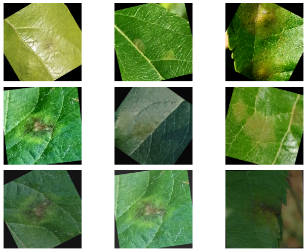
We can see that this will make the dataset harder but will also help the model to learn more features.

The validation transforms only convert the images to tensors and normalize them. For normalization, we are using the ImageNet mean and standard deviation as we will be using a pretrained model.

The Datasets and Data Loaders

The next function prepares the training and validation datasets.

def get_datasets():
    """
    Function to prepare the Datasets.
    Returns the training and validation datasets along 
    with the class names.
    """
    dataset = datasets.ImageFolder(
        ROOT_DIR, 
        transform=(get_train_transform(IMAGE_SIZE))
    )
    dataset_test = datasets.ImageFolder(
        ROOT_DIR, 
        transform=(get_valid_transform(IMAGE_SIZE))
    )
    dataset_size = len(dataset)

    # Calculate the validation dataset size.
    valid_size = int(VALID_SPLIT*dataset_size)
    # Radomize the data indices.
    indices = torch.randperm(len(dataset)).tolist()
    # Training and validation sets.
    dataset_train = Subset(dataset, indices[:-valid_size])
    dataset_valid = Subset(dataset_test, indices[-valid_size:])

    return dataset_train, dataset_valid, dataset.classes

As the images are already in their class folders, we can use the ImageFolder class. Also, we are using the SubSet class to create the validation set out of the same ImageFolder instance.

Next is the function to prepare the data loaders.

def get_data_loaders(dataset_train, dataset_valid):
    """
    Prepares the training and validation data loaders.
    :param dataset_train: The training dataset.
    :param dataset_valid: The validation dataset.
    Returns the training and validation data loaders.
    """
    train_loader = DataLoader(
        dataset_train, batch_size=BATCH_SIZE, 
        shuffle=True, num_workers=NUM_WORKERS
    )
    valid_loader = DataLoader(
        dataset_valid, batch_size=BATCH_SIZE, 
        shuffle=False, num_workers=NUM_WORKERS
    )
    return train_loader, valid_loader 

It accepts the datasets and returns the respective data loaders.

The ResNet34 Image Classification Model

For early apple scab recognition, we are going to fine tune a ResNet34 model pretrained on the ImageNet dataset.

The model.py file will hold the code for this.

import torch.nn as nn

from torchvision import models

def build_model(pretrained=True, fine_tune=True, num_classes=10):
    if pretrained:
        print('[INFO]: Loading pre-trained weights')
        model = models.resnet34(weights='DEFAULT')
    else:
        print('[INFO]: Not loading pre-trained weights')
        model = models.resnet34(weights=None)
        
    if fine_tune:
        print('[INFO]: Fine-tuning all layers...')
        for params in model.parameters():
            params.requires_grad = True
    elif not fine_tune:
        print('[INFO]: Freezing hidden layers...')
        for params in model.parameters():
            params.requires_grad = False

    # Change the final classification head.
    model.fc = nn.Linear(in_features=512, out_features=num_classes)
    return model

Note: Starting from PyTorch 1.12.0, the pretrained argument is deprecated. To load the best ImageNet weights we have to use the weights argument and pass the value as 'DEFAULT'. It will load the best ImageNet weights, either IMAGENET1K_V1 or IMAGENET1K_V2.

Also, note that we are changing the number of out_features according to the number of classes in the dataset. With this, we complete the model preparation code as well.

The Training Script

We need an executable Python script that will drive the entire training procedure by combining all the modules that we have seen till now.

We will use the train.py file for this.

Here, we will go over the code for the training script in brief.

First, the import statements and defining the argument parsers.

import torch
import argparse
import torch.nn as nn
import torch.optim as optim
import time

from tqdm.auto import tqdm

from model import build_model
from datasets import get_datasets, get_data_loaders
from utils import save_model, save_plots, SaveBestModel

seed = 42
torch.manual_seed(seed)
torch.cuda.manual_seed(seed)
torch.backends.cudnn.deterministic = True
torch.backends.cudnn.benchmark = True

# Construct the argument parser.
parser = argparse.ArgumentParser()
parser.add_argument(
    '-e', '--epochs', type=int, default=10,
    help='Number of epochs to train our network for'
)
parser.add_argument(
    '-lr', '--learning-rate', type=float,
    dest='learning_rate', default=0.001,
    help='Learning rate for training the model'
)
args = vars(parser.parse_args())

Along with the imports, we are also setting the seed for reproducible results on a particular system.

We have two flags for the argument parser. One is to pass the number of epochs to train for, and another one is to control the learning rate of the optimizer.

Next are the training and validation functions.

# Training function.
def train(model, trainloader, optimizer, criterion):
    model.train()
    print('Training')
    train_running_loss = 0.0
    train_running_correct = 0
    counter = 0
    for i, data in tqdm(enumerate(trainloader), total=len(trainloader)):
        counter += 1
        image, labels = data
        image = image.to(device)
        labels = labels.to(device)
        optimizer.zero_grad()
        # Forward pass.
        outputs = model(image)
        # Calculate the loss.
        loss = criterion(outputs, labels)
        train_running_loss += loss.item()
        # Calculate the accuracy.
        _, preds = torch.max(outputs.data, 1)
        train_running_correct += (preds == labels).sum().item()
        # Backpropagation.
        loss.backward()
        # Update the weights.
        optimizer.step()
    
    # Loss and accuracy for the complete epoch.
    epoch_loss = train_running_loss / counter
    epoch_acc = 100. * (train_running_correct / len(trainloader.dataset))
    return epoch_loss, epoch_acc

# Validation function.
def validate(model, testloader, criterion, class_names):
    model.eval()
    print('Validation')
    valid_running_loss = 0.0
    valid_running_correct = 0
    counter = 0

    with torch.no_grad():
        for i, data in tqdm(enumerate(testloader), total=len(testloader)):
            counter += 1
            
            image, labels = data
            image = image.to(device)
            labels = labels.to(device)
            # Forward pass.
            outputs = model(image)
            # Calculate the loss.
            loss = criterion(outputs, labels)
            valid_running_loss += loss.item()
            # Calculate the accuracy.
            _, preds = torch.max(outputs.data, 1)
            valid_running_correct += (preds == labels).sum().item()
        
    # Loss and accuracy for the complete epoch.
    epoch_loss = valid_running_loss / counter
    epoch_acc = 100. * (valid_running_correct / len(testloader.dataset))
    return epoch_loss, epoch_acc

The above train and validate functions are very general image classification functions in PyTorch. They are almost similar. The only difference is that the validation function does not involve backpropagation. Other than that, both of them return the loss and accuracy values for each epoch.

Finally, we have the main code block.

if __name__ == '__main__':
    # Load the training and validation datasets.
    dataset_train, dataset_valid, dataset_classes = get_datasets()
    print(f"[INFO]: Number of training images: {len(dataset_train)}")
    print(f"[INFO]: Number of validation images: {len(dataset_valid)}")
    print(f"[INFO]: Classes: {dataset_classes}")
    # Load the training and validation data loaders.
    train_loader, valid_loader = get_data_loaders(dataset_train, dataset_valid)

    # Learning_parameters. 
    lr = args['learning_rate']
    epochs = args['epochs']
    device = ('cuda' if torch.cuda.is_available() else 'cpu')
    print(f"Computation device: {device}")
    print(f"Learning rate: {lr}")
    print(f"Epochs to train for: {epochs}\n")

    # Load the model.
    model = build_model(
        pretrained=True,
        fine_tune=True, 
        num_classes=len(dataset_classes)
    ).to(device)
    
    # Total parameters and trainable parameters.
    total_params = sum(p.numel() for p in model.parameters())
    print(f"{total_params:,} total parameters.")
    total_trainable_params = sum(
        p.numel() for p in model.parameters() if p.requires_grad)
    print(f"{total_trainable_params:,} training parameters.")

    # Optimizer.
    optimizer = optim.SGD(model.parameters(), lr=lr, momentum=0.9)
    # Loss function.
    criterion = nn.CrossEntropyLoss()

    # Initialize `SaveBestModel` class.
    save_best_model = SaveBestModel()

    # Lists to keep track of losses and accuracies.
    train_loss, valid_loss = [], []
    train_acc, valid_acc = [], []
    # Start the training.
    for epoch in range(epochs):
        print(f"[INFO]: Epoch {epoch+1} of {epochs}")
        train_epoch_loss, train_epoch_acc = train(model, train_loader, 
                                                optimizer, criterion)
        valid_epoch_loss, valid_epoch_acc = validate(model, valid_loader,  
                                                    criterion, dataset_classes)
        train_loss.append(train_epoch_loss)
        valid_loss.append(valid_epoch_loss)
        train_acc.append(train_epoch_acc)
        valid_acc.append(valid_epoch_acc)
        print(f"Training loss: {train_epoch_loss:.3f}, training acc: {train_epoch_acc:.3f}")
        print(f"Validation loss: {valid_epoch_loss:.3f}, validation acc: {valid_epoch_acc:.3f}")
        save_best_model(valid_epoch_loss, epoch, model)
        print('-'*50)

    # Save the trained model weights.
    save_model(epochs, model, optimizer, criterion)
    # Save the loss and accuracy plots.
    save_plots(train_acc, valid_acc, train_loss, valid_loss)
    print('TRAINING COMPLETE')

We create the datasets, and the data loaders, initialize the model with the pretrained weights and define the optimizer & loss function also. We also initialize the SaveBestModel class and create four lists to store the accuracy and loss values. After each epoch, we print the metrics and the loss and save the best model if the validation loss for that epoch is the lowest.

At end of the training, we save the final model and the loss & accuracy graphs.

This completes the entire training script.

Training the ResNet34 Model for Early Apple Scab Recognition

We are all set with the code files that need to start the training.

Note: All the experiments in this tutorial were carried out on a machine with a 10GB RTX 3080 GPU, 32 GB RAM, and an i7 10th generation CPU.

Execute the following command on the terminal within src directory to start the training.

python train.py --epochs 50 -lr 0.0005

We are training the ResNet34 model for 50 epochs with 0.0005 learning rate.

The following block shows the truncated output from the terminal.

[INFO]: Number of training images: 1683
[INFO]: Number of validation images: 296
[INFO]: Classes: ['Background', 'Healthy', 'Scab']
Computation device: cuda
Learning rate: 0.0005
Epochs to train for: 50

[INFO]: Loading pre-trained weights
[INFO]: Fine-tuning all layers...
21,286,211 total parameters.
21,286,211 training parameters.
[INFO]: Epoch 1 of 50
Training
100%|████████████████████████████████████████████████████████████████████████████████| 106/106 [00:17<00:00,  6.21it/s]
Validation
100%|██████████████████████████████████████████████████████████████████████████████████| 19/19 [00:01<00:00, 14.56it/s]
Training loss: 0.597, training acc: 75.104
Validation loss: 0.300, validation acc: 89.189

Best validation loss: 0.3002579996460362

Saving best model for epoch: 1
.
.
.
[INFO]: Epoch 50 of 50
Training
100%|████████████████████████████████████████████████████████████████████████████████| 106/106 [00:13<00:00,  8.11it/s]
Validation
100%|██████████████████████████████████████████████████████████████████████████████████| 19/19 [00:01<00:00, 17.92it/s]
Training loss: 0.016, training acc: 99.703
Validation loss: 0.041, validation acc: 98.649
--------------------------------------------------
TRAINING COMPLETE

By the end of the training, we have over 98% validation accuracy.

To get a better idea of how the training process went, we can take a look at the accuracy and loss plots.

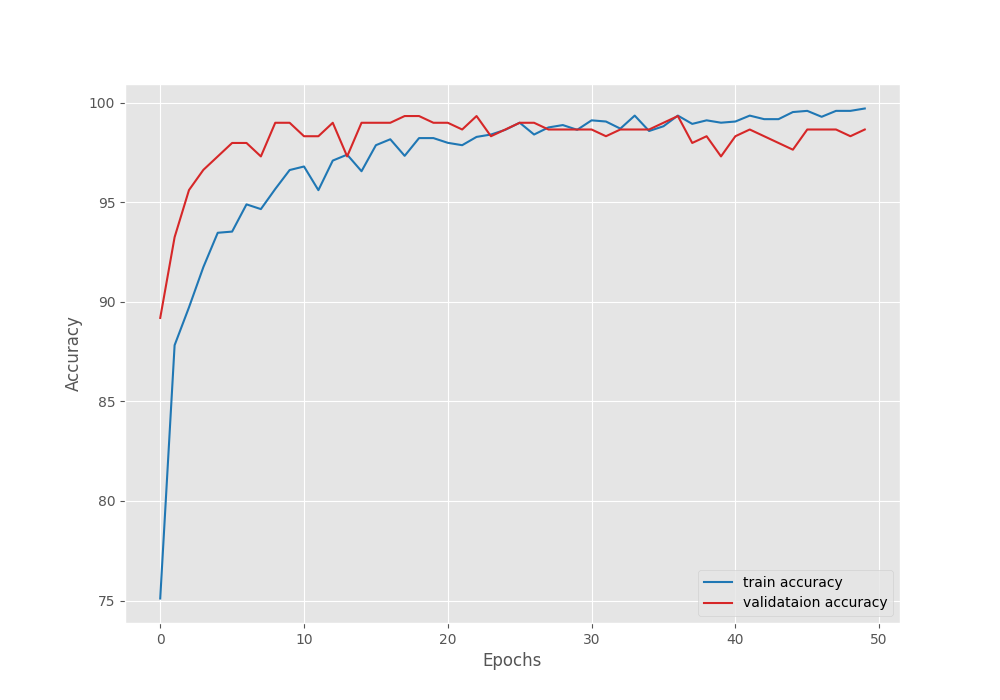
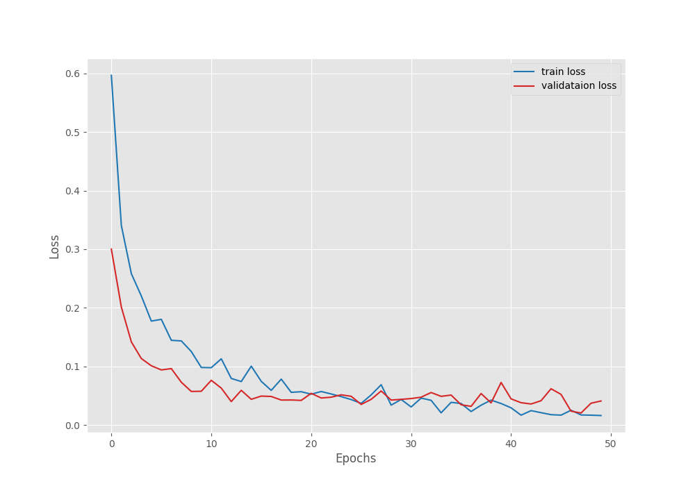
From the validation loss graph, it looks like the models started to overfit around epoch 37. We can also see the validation accuracy value decreasing around that point. It is a good thing that we were saving the best model weights as well. Else, we would have got an overfit model.

In case, you want to train longer without overfitting the model, try out more augmentation techniques, or even use a learning rate scheduler after 35 epochs. These steps will surely help.

Testing the Trained Model

To evaluate our model properly, we can test it on the held-out test set that we prepared earlier.

The test script is going to be very simple. Although we will not go into the details of the test code explanation, the following few blocks contain the entire code for the test script.

All the code for testing the model will go into the test.py file.

The following code block imports the necessary packages and defines a few constants.

import torch
import numpy as np
import cv2
import os
import torch.nn.functional as F
import torchvision.transforms as transforms

from tqdm.auto import tqdm
from model import build_model
from torch.utils.data import DataLoader
from torchvision import datasets

# Constants and other configurations.
TEST_DIR = os.path.join('..', 'input', 'test')
BATCH_SIZE = 1
DEVICE = torch.device('cuda:0' if torch.cuda.is_available() else 'cpu')
IMAGE_RESIZE = 512
NUM_WORKERS = 4
CLASS_NAMES = ['Background', 'Healthy', 'Scab']

Be sure to use the same resizing factor as was in the training procedure, in case you change it during training.

The next three functions define the transforms, prepare the dataset, and the data loader.

# Validation transforms
def get_test_transform(image_size):
    test_transform = transforms.Compose([
        transforms.Resize((image_size, image_size)),
        transforms.ToTensor(),
        transforms.Normalize(
            mean=[0.485, 0.456, 0.406],
            std=[0.229, 0.224, 0.225]
            )
    ])
    return test_transform

def get_datasets(image_size):
    """
    Function to prepare the Datasets.
    Returns the test dataset.
    """
    dataset_test = datasets.ImageFolder(
        TEST_DIR, 
        transform=(get_test_transform(image_size))
    )
    return dataset_test

def get_data_loader(dataset_test):
    """
    Prepares the training and validation data loaders.
    :param dataset_test: The test dataset.

    Returns the training and validation data loaders.
    """
    test_loader = DataLoader(
        dataset_test, batch_size=BATCH_SIZE, 
        shuffle=False, num_workers=NUM_WORKERS
    )
    return test_loader

We will also save the image results by annotating them with the ground truth and predictions. The following two functions help us with that.

def denormalize(
    x, 
    mean=[0.485, 0.456, 0.406], 
    std=[0.229, 0.224, 0.225]
):
    for t, m, s in zip(x, mean, std):
        t.mul_(s).add_(m)
    return torch.clamp(x, 0, 1)

def save_test_results(
    tensor, 
    target, 
    output_class, 
    counter, 
    test_result_save_dir
):
    """
    This function will save a few test images along with the 
    ground truth label and predicted label annotated on the image.

    :param tensor: The image tensor.
    :param target: The ground truth class number.
    :param output_class: The predicted class number.
    :param counter: The test image number.
    """
    image = denormalize(tensor).cpu()
    image = image.squeeze(0).permute((1, 2, 0)).numpy()
    image = np.ascontiguousarray(image, dtype=np.float32)
    image = cv2.cvtColor(image, cv2.COLOR_RGB2BGR)
    gt = target.cpu().numpy()
    cv2.putText(
        image, f"GT: {CLASS_NAMES[int(gt)]}", 
        (5, 25), cv2.FONT_HERSHEY_SIMPLEX, 
        0.6, (0, 255, 0), 2, cv2.LINE_AA
    )
    if output_class == gt:
        color = (0, 255, 0)
    else:
        color = (0, 0, 255)
    cv2.putText(
        image, f"Pred: {CLASS_NAMES[int(output_class)]}", 
        (5, 55), cv2.FONT_HERSHEY_SIMPLEX, 
        0.6, color, 2, cv2.LINE_AA
    )
    cv2.imwrite(
        os.path.join(test_result_save_dir, 'test_image_'+str(counter)+'.png'), 
        image*255.
    )

Now, the function that does the testing.

def test(model, testloader, device, test_result_save_dir):
    """
    Function to test the trained model on the test dataset.

    :param model: The trained model.
    :param testloader: The test data loader.
    :param device: The computation device.
    :param test_result_save_dir: Path to save the resulting images.

    Returns:
        predictions_list: List containing all the predicted class numbers.
        ground_truth_list: List containing all the ground truth class numbers.
        acc: The test accuracy.
    """
    model.eval()
    print('Testing model')
    predictions_list = []
    ground_truth_list = []
    test_running_correct = 0
    counter = 0
    with torch.no_grad():
        for i, data in tqdm(enumerate(testloader), total=len(testloader)):
            counter += 1
            image, labels = data
            image = image.to(device)
            labels = labels.to(device)

            # Forward pass.
            outputs = model(image)
            # Softmax probabilities.
            predictions = torch.softmax(outputs, dim=1).cpu().numpy()
            # Predicted class number.
            output_class = np.argmax(predictions)
            # Append the GT and predictions to the respective lists.
            predictions_list.append(output_class)
            ground_truth_list.append(labels.cpu().numpy())
            # Calculate the accuracy.
            _, preds = torch.max(outputs.data, 1)
            test_running_correct += (preds == labels).sum().item()

            save_test_results(
                image, 
                labels,
                output_class, 
                counter, 
                test_result_save_dir
            )

    acc = 100. * (test_running_correct / len(testloader.dataset))
    return predictions_list, ground_truth_list, acc

Finally, the main code block to start the testing.

if __name__ == '__main__':
    test_result_save_dir = os.path.join('..', 'outputs', 'test_results')
    os.makedirs(test_result_save_dir, exist_ok=True)

    dataset_test = get_datasets(IMAGE_RESIZE)
    test_loader = get_data_loader(dataset_test)

    checkpoint = torch.load(os.path.join('..', 'outputs', 'best_model.pth'))
    # Load the model.
    model = build_model(
        pretrained=False,
        fine_tune=False, 
        num_classes=len(CLASS_NAMES)
    ).to(DEVICE)
    model.load_state_dict(checkpoint['model_state_dict'])
    predictions_list, ground_truth_list, acc = test(
        model, 
        test_loader, 
        DEVICE,
        test_result_save_dir
    )
    print(f"Test accuracy: {acc:.3f}%")

Execute the following command in the terminal to test the model.

python test.py 

The following the is output.

[INFO]: Not loading pre-trained weights
[INFO]: Freezing hidden layers...
Testing model
100%|████████████████████████████████████████████████████████████████████████████████| 192/192 [00:05<00:00, 37.38it/s]
Test accuracy: 98.958%

We are getting over 98% accuracy. Out of the 192 images, only two predictions are incorrect. The results are saved in the outputs/test_results directory.

The following figure shows the two incorrect predictions.

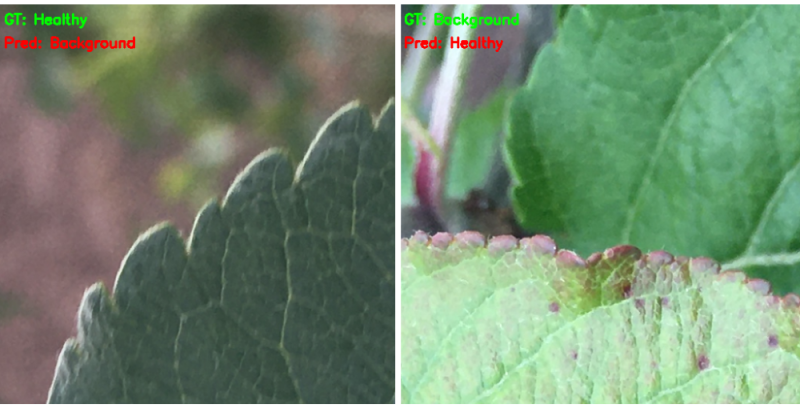
In one of the cases, it is predicting a Background class as Healthy and in another, it is predicting Healthy as Background.

But as we can see from the images, the ground truth themselves is ambiguous. It is pretty difficult to figure out whether the images belong to the Background or Healthy class.

Visualizing Class Activation Maps

In the testing phase, we were able to figure out the wrong predictions. But we could not know which area of an image the model was looking at while making the predictions.

Even if the model is predicting a leaf with an early scab correctly, then is it really looking at the scab?

We can answer these questions by looking at the class activation maps. The codebase (downloadable zip file) contains a cam.py script that shows the class activation map of the model for each test image.

The cam.py script is already included as part of the downloadable zip file.

Let’s execute the cam.py script.

python cam.py 

All the image outputs along with the class activation maps will be available in the outputs/cam_results directory.

The following are the two wrong predictions that we saw earlier.

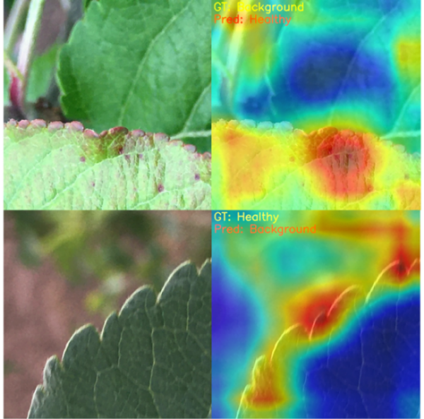
We can see that in the first case it is looking at the leaves (which are healthy) to predict the class as Healthy instead of Background. In the second case, it is mostly looking at the background. From the model’s perspective, the predictions do not look wrong.

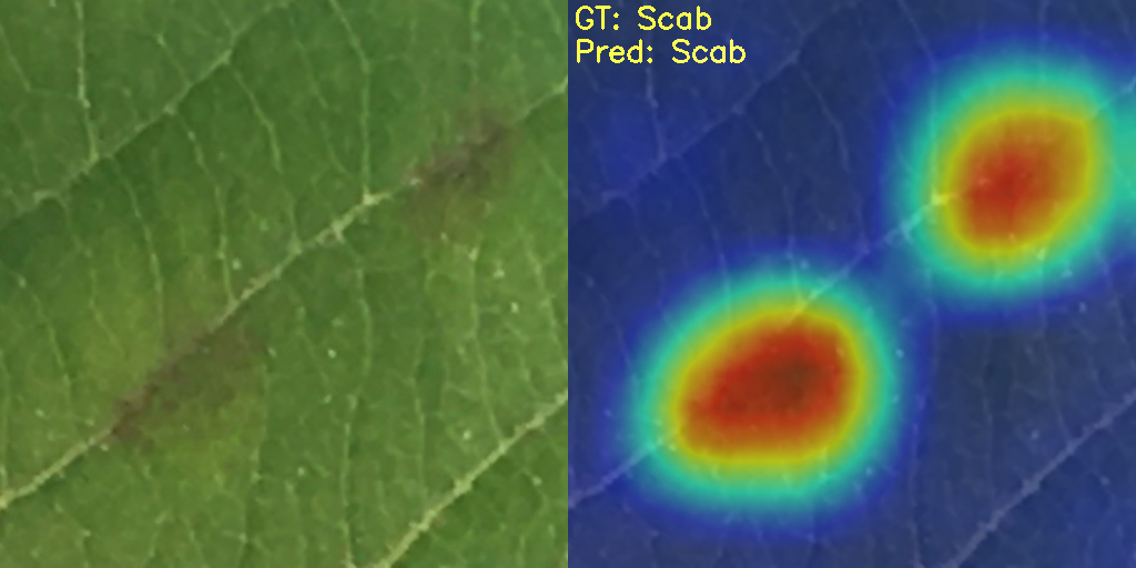
Taking a look at the right predictions will also give us a pretty good idea about the model’s predictions.

It is quite clear that the model is looking at all the places on the leaves which are affected by the early scab disease. In fact, it is able to detect those early scabs as well which are not clearly visible to the naked eye.

Takeaway

From this tutorial, we can be sure that using deep learning and computer vision for plant pathology is a good idea. It is very surprising how accurate the ResNet34 model was in detecting even the difficult early scab disease spots.

If you expand this project in any way, let others know in the comment section.

Summary and Conclusion

In this blog post, we carried out early scab recognition in apple leaves using a ResNet34 model. We employed the PyTorch deep learning framework for this. We also observed how class activation maps can help us decode why the model made a certain prediction. I hope that you found this post useful.

If you have any doubts, thoughts, or suggestions, please leave them in the comment section. I will surely address them.

You can contact me using the Contact section. You can also find me on LinkedIn, and Twitter.