
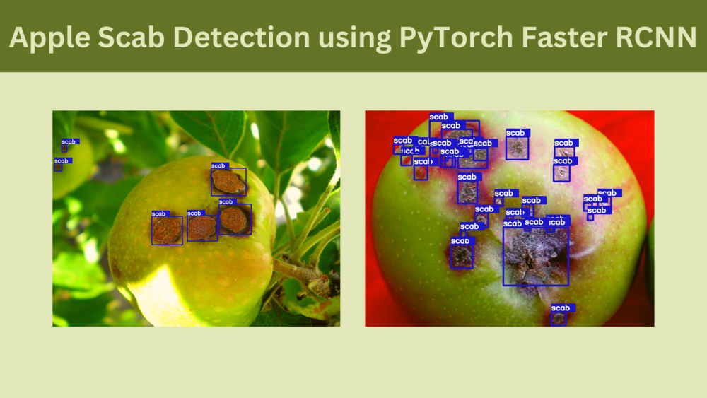
When dealing with plant pathology using deep learning, sometimes, image recognition is not enough. One such example is the identification of the apple scab disease. The last two blog posts covered the recognition of apple scab in leaves and fruits. In the apple fruit, pinpointing where the actual disease is, will be more helpful. Extending our “deep learning for plant pathology” series, in this tutorial, we will use PyTorch Faster RCNN for apple scab detection.
Using object detection for apple scab detection will solve two problems for us that image recognition could not.
- When using image recognition for apple scab identification, the model was only able to tell whether the leaf or fruit has been affected by the disease or not. Then we had to analyze the image manually to check which part of the leaf or fruit the disease is affecting.
- When using object detection for apple scab detection, the model will already give us the localization predictions. We just need to look at those specific places and confirm whether the apple scab disease is present or not. This is going to be much more convenient.
Let’s check out the topics that we will cover in this tutorial:
- We will start with exploring the apple scab detection dataset.
- Then we will move to the discussion of the code and model that we will use for object detection.
- We will use the Faster RCNN ResNet FPN V2 PyTorch model for training.
- After the training, we will analyze the results.
- Next, we will carry out inference using some videos from the internet for apple scab detection.
- Finally, we will finish the tutorial by discussing the improvements that we can add to this project.
Let’s jump into the details without any further delay.
Preparing the Apple Scab Detection Dataset
We start with the AppeScabFDs dataset from Kaggle to prepare the apple scab detection dataset.
We also used this dataset for apple fruit scab recognition in the previous post.
But as we know, this dataset only supports image classification out of the box.
So, how do we prepare it for detection?
We have to go through the manual and tedious process of annotating the image ourselves. But for this project, the annotation of the images has already been done.
LabelImg was used to annotate the scab regions of the apples (207 images) and create the annotation files in Pascal VOC XML format.
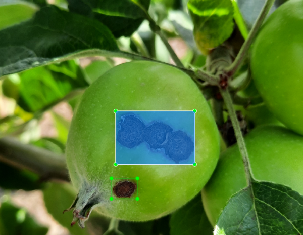
It is important to note that we only use the images under the Scab directory because in object detection we only need the true positives while annotating the images.
The final dataset is available here on Kaggle. The dataset has already been split into 183 training images and 24 validation images.
The following are a few images with the ground truth annotations from the final training set.
You may go ahead and download the dataset for now. In the next section, we will check how to structure the entire project directory.
Directory Structure
The following block shows the directory structure for the entire project.
├── data
│   ├── apple_scab_detection
│   │   ├── train_images
│   │   ├── train_labels
│   │   ├── valid_images
│   │   └── valid_labels
│   └── inference_data
│       ├── video_1.mp4
│       └── video_1_trimmed.mp4
├── data_configs
│   └── apple_scab.yaml
├── datasets.py
├── inference.py
├── inference_video.py
├── models
│   ├── create_fasterrcnn_model.py
│   ├── fasterrcnn_resnet50_fpn.py
│   ├── fasterrcnn_resnet50_fpn_v2.py
│   └── __init__.py
├── notebooks
│   └── visualizations.ipynb
├── outputs
│   ├── inference
│   │   └── res_1
│   └── training
│       └── epochs50_allaug
├── random_split.py
├── README.md
├── requirements.txt
├── torch_utils
│   ├── coco_eval.py
│   ├── coco_utils.py
│   ├── engine.py
│   ├── __init__.py
│   ├── README.md
│   └── utils.py
├── train.py
└── utils
    ├── annotations.py
    ├── general.py
    ├── __init__.py
    ├── logging.py
    └── transforms.py
- The
datadirectory contains theapple_scab_detectionsubdirectory with the training & validation images as well as the XML annotation files. We also have aninference_datasubdirectory with any images or videos that we will like to carry out inference on. - The
data_configdirectory contains a YAML file holding all the dataset and class information. - Other than that we have several scripts for training, inference, and utility functions.
- The
train.pyis the driver script that we will use for training.
All the code files along with the proper structure are available for download. To run the training locally, you just need to download the dataset and arrange it in the above structure.
The Object Detection Codebase
We are not going into too many details about the object detection codebase here. This is a smaller part of a much larger project that you can find here on GitHub.
We have removed all the parts that we do not need for the apple scab detection training.
Still, if you want to get into the details, the repository is the best place to do so.
You can also go through the Fine Tuning Faster RCNN ResNet50 FPN V2 post to get a few more details.
Download Code
Installing the Requirements
If you are on Linux, you can just install the requirements from the requirements.txt file to get started right away.
pip install -r requirements.txt
For Windows OS, you may need to follow these instructions so that you can set up the pycocotools (for mAP calculation) correctly.
The Augmentations Applied to the Apple Scab Detection Dataset
The dataset does not contain too many images. We have just 183 images for training and 24 for validation.
We have to get the most out of what we have. Using extensive image augmentation can introduce enough variability into the dataset.
Fortunately, the code that we use supports mosaic augmentations and several other albumentations based augmentations.
Take a look at the following image. It shows how a single image looks when 4 images are combined using mosaic augmentation and all the other augmentations are also applied.
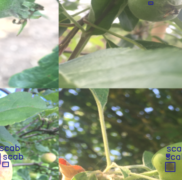
In mosaic augmentation, we combine four images by cropping them in different ratios. This has proved to be very beneficial for training object detection models.
Training the Faster RCNN ResNet FPN V2 model for Apple Scab Detection
Let’s get into the training part of this tutorial.
All the training and inference experiments in this tutorial have been conducted on a machine with 10 GB RTX 3080 GPU, 32 GB of RAM, and an i7 10th generation processor.
The training and inference scripts have been arranged in a very simple manner.
To start the training, execute the following command within the project directory.
python train.py \
--model fasterrcnn_resnet50_fpn_v2 \
--batch 4 \
--epochs 50 \
--use-train-aug \
--data data_configs/apple_scab.yaml \
--name epochs50_allaug
Let’s go over all the command line arguments.
--model: This takes a key value to inform the training script which model to use. This code base supportsfasterrcnn_resnet50_fpn_v2(new model) andfasterrcnn_resnet50_fpn. Here, we are using the newer Faster RCNN ResNet50 FPN V2 model as it gives better results.--batch: The training and validation batch size here is 4. This consumes around 8 GB of VRAM with 640×640 resolution training images. If you are training locally and face OOM (Out Of Memory) error, please consider reducing the batch size to 2.--epochs: We are training the model for 50 epochs.--use-train-aug: By default, the training script uses mosaic augmentation. Along with that, we are also passing this boolean flag that tells the script to use the additional augmentations.--data: This flag accepts the path to the dataset YAML file. The YAML file contains the path to images, annotation, class names, and the number of classes.--name: We can provide an explanatory project name using this flag. This will create a subdirectory underoutputs/trainingdirectory using the same name. It helps to easily differentiate between different training experiments.
The following is the truncated output from the final epoch.
Epoch: [49]  [ 0/45]  eta: 0:02:46  lr: 0.001000  loss: 0.5461 (0.5461)  loss_classifier: 0.1044 (0.1044)  loss_box_reg: 0.2099 (0.2099)  loss_objectness: 0.0374 (0.0374)  loss_rpn_box_reg: 0.1944 (0.1944)  time: 3.6905  data: 3.3475  max mem: 5192
Epoch: [49]  [44/45]  eta: 0:00:00  lr: 0.001000  loss: 0.4430 (0.4158)  loss_classifier: 0.0815 (0.0777)  loss_box_reg: 0.1998 (0.1888)  loss_objectness: 0.0209 (0.0365)  loss_rpn_box_reg: 0.1209 (0.1128)  time: 0.7624  data: 0.4315  max mem: 5192
Epoch: [49] Total time: 0:00:39 (0.8671 s / it)
Test:  [0/6]  eta: 0:00:05  model_time: 0.1414 (0.1414)  evaluator_time: 0.0038 (0.0038)  time: 0.9233  data: 0.7348  max mem: 5192
Test:  [5/6]  eta: 0:00:00  model_time: 0.1357 (0.1267)  evaluator_time: 0.0046 (0.0055)  time: 0.2663  data: 0.1250  max mem: 5192
Test: Total time: 0:00:01 (0.2734 s / it)
Average Precision  (AP) @[ IoU=0.50:0.95 | area=   all | maxDets=100 ] = 0.37435535204021597
Average Precision  (AP) @[ IoU=0.50      | area=   all | maxDets=100 ] = 0.7532503816294729
Average Precision  (AP) @[ IoU=0.75      | area=   all | maxDets=100 ] = 0.36091233591814287
Average Precision  (AP) @[ IoU=0.50:0.95 | area= small | maxDets=100 ] = 0.3300101898839323
Average Precision  (AP) @[ IoU=0.50:0.95 | area=medium | maxDets=100 ] = 0.6437478033517637
Average Precision  (AP) @[ IoU=0.50:0.95 | area= large | maxDets=100 ] = 0.7267326732673267
Average Recall     (AR) @[ IoU=0.50:0.95 | area=   all | maxDets=  1 ] = 0.09318181818181817
Average Recall     (AR) @[ IoU=0.50:0.95 | area=   all | maxDets= 10 ] = 0.38636363636363635
Average Recall     (AR) @[ IoU=0.50:0.95 | area=   all | maxDets=100 ] = 0.421969696969697
Average Recall     (AR) @[ IoU=0.50:0.95 | area= small | maxDets=100 ] = 0.37345132743362836
Average Recall     (AR) @[ IoU=0.50:0.95 | area=medium | maxDets=100 ] = 0.7066666666666667
Average Recall     (AR) @[ IoU=0.50:0.95 | area= large | maxDets=100 ] = 0.725
But this was not the best epoch. The following are the mAP results from the best epoch, epoch 43 (the terminal outputs epoch number starting from 0, so, 0 to 49 in our case).
Epoch: [42]  [ 0/45]  eta: 0:02:42  lr: 0.001000  loss: 0.3858 (0.3858)  loss_classifier: 0.0758 (0.0758)  loss_box_reg: 0.1718 (0.1718)  loss_objectness: 0.0257 (0.0257)  loss_rpn_box_reg: 0.1126 (0.1126)  time: 3.6103  data: 3.2708  max mem: 5192
Epoch: [42]  [44/45]  eta: 0:00:00  lr: 0.001000  loss: 0.3600 (0.3937)  loss_classifier: 0.0736 (0.0759)  loss_box_reg: 0.1703 (0.1731)  loss_objectness: 0.0260 (0.0334)  loss_rpn_box_reg: 0.0799 (0.1113)  time: 0.7689  data: 0.4379  max mem: 5192
Epoch: [42] Total time: 0:00:38 (0.8563 s / it)
Test:  [0/6]  eta: 0:00:05  model_time: 0.1430 (0.1430)  evaluator_time: 0.0046 (0.0046)  time: 0.9220  data: 0.7387  max mem: 5192
Test:  [5/6]  eta: 0:00:00  model_time: 0.1367 (0.1274)  evaluator_time: 0.0047 (0.0058)  time: 0.2666  data: 0.1256  max mem: 5192
Test: Total time: 0:00:01 (0.2740 s / it)
Average Precision  (AP) @[ IoU=0.50:0.95 | area=   all | maxDets=100 ] = 0.3861075990416181
Average Precision  (AP) @[ IoU=0.50      | area=   all | maxDets=100 ] = 0.7561515998822166
Average Precision  (AP) @[ IoU=0.75      | area=   all | maxDets=100 ] = 0.3918785457208387
Average Precision  (AP) @[ IoU=0.50:0.95 | area= small | maxDets=100 ] = 0.3409863155683963
Average Precision  (AP) @[ IoU=0.50:0.95 | area=medium | maxDets=100 ] = 0.6417609618104668
Average Precision  (AP) @[ IoU=0.50:0.95 | area= large | maxDets=100 ] = 0.6937293729372936
Average Recall     (AR) @[ IoU=0.50:0.95 | area=   all | maxDets=  1 ] = 0.10378787878787879
Average Recall     (AR) @[ IoU=0.50:0.95 | area=   all | maxDets= 10 ] = 0.39696969696969703
Average Recall     (AR) @[ IoU=0.50:0.95 | area=   all | maxDets=100 ] = 0.4340909090909091
Average Recall     (AR) @[ IoU=0.50:0.95 | area= small | maxDets=100 ] = 0.3893805309734513
Average Recall     (AR) @[ IoU=0.50:0.95 | area=medium | maxDets=100 ] = 0.7
Average Recall     (AR) @[ IoU=0.50:0.95 | area= large | maxDets=100 ] = 0.7
We have the best model in the outputs/training/epochs50_allaug directory according to the best mAP object detection metrics. Along with that, the training script also stores several loss and mAP graphs.
Analyzing the Results
The following are the mAP graphs from the validation loop.
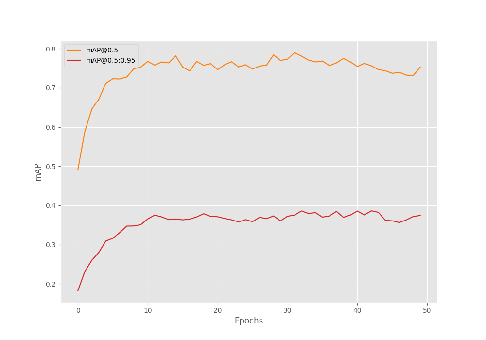
From the mAP graph (both, at 0.50 IoU and at 0.50:0.95 IoU), we can also see some indications of overfitting at the end.
However, this should not concern us much. Given the small size of the dataset, this is expected. Further, as we are saving the best model weights, we will use those for inference. So, we need not worry about any overfit model issue.
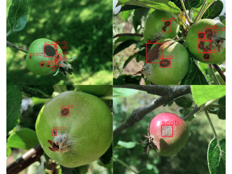
During training, the script also stores the predictions of a few images from the validation data on each epoch. Let’s take a look at them first before moving to the inference part.
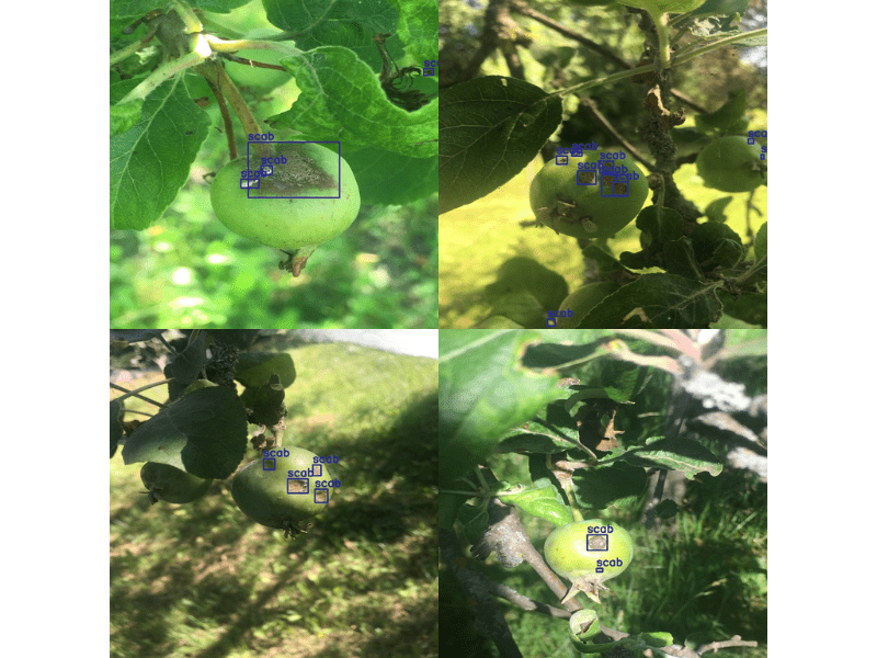
In the above image, the model is detecting the apple scab regions correctly, apart from one image. In one of the images, the model is detecting the scab disease on the leaf.
Inference on Images for Apple Scab Detection
Carrying out inference on images is pretty easy. We can use the inference.py and just provide the directory path where all the images are present.
There are four images present in the data/inference_data directory which were neither part of the training set nor the validation set. They are random images from the internet.
We can run inference on these images by executing the following command.
python inference.py \
--weights outputs/training/epochs50_allaug/best_model.pth \
--input data/inference_data/
The following are the results.

The first image (top-left) has a very blurry apple at the back. Still, the model was able to detect the scab disease on it. It is really impressive.
But for the image in the top-right corner, the model is making a few mistakes. It is detecting some scab disease regions on the leaves at the corners.
The next image (bottom-right) is pretty easy and the model is detecting all the scab regions pretty well.
In the final image (bottom-left) also the model predicts all the regions affected by the scab disease correctly.
Looks like even though we had very few images for training, the Faster RCNN ResNet50 FPN V2 is quite capable of learning all the necessary features.
Inference on Videos using the Trained Faster RCNN ResNet50 FPN V2
For the final testing of the model, we will run inference on a quite challenging video from YouTube.
It is a very fast-moving video with most of the frame out of focus. The original video has been trimmed down so that apples with scab diseases are present in most of the frames.
To run inference on videos, we need to execute the following command. You can provide the path to your own video to run inference on videos.
python inference_video.py \
--weights outputs/training/epochs50_allaug/best_model.pth \
--input data/inference_data/video_2_part1.mp4 \
--show
There are two major observations here:
- The model is able to detect almost all of the scab disease regions on the apples.
- Yet, the number of false positives is high. The model is detecting patches on leaves as well as on the background which look like the apple scab disease.
What may be the reason for the second observation? Remember that we are using mosaic augmentation which crops the images and stitches them together. In this process, some of the background information from the original image is lost. When training on the mosaic images, the model does not get to see blurry backgrounds with patches which it should not focus on.
Moreover, the objects that we want to detect here are quite small. In most real-life scenarios the background will cover a major area. This shows one case where mosaic augmentation does not work very well in object detection. Most probably, training just with the simple object detection augmentations applied to the entire image will be more helpful for the model. But we are keeping that experiment for a future post.
Further Improvements
We can take this project a notch up. Along with predicting the bounding boxes for the apple scab disease on the fruits, we can do so for the leaves as well. This will again require annotating a lot of images of apple leaves with scab disease.
But after the entire project is done, it will be really nice to have a single model for apple scab disease detection of both leaves and fruits.
Summary and Conclusion
In this blog post, we carried out apple scab detection using the PyTorch Faster RCNN ResNet50 FPN V2 model. We started with the dataset discussion, moved on to the code base discussion, and then trained the model. We also ran inference on images and videos which gave us more insights. This experiment also proved that all the augmentation techniques may not be beneficial when trying to detect small objects with a lot of background. Hopefully, this was a good learning experience for you.
If you have any doubts, thoughts, or suggestions, please leave them in the comment section. I will surely address them.
You can contact me using the Contact section. You can also find me on LinkedIn, and X.
Images / Videos Credits Used for Inference
image_1.png: https://www.agric.wa.gov.au/pome-fruit/managing-apple-scab-western-australiaimage_2.jpg: https://www.onlinepestcontrol.com/apple-scab-and-treatment/image_3.jpg: http://applescout.ca.uky.edu/scabimage_4.jpg: https://ca.decisionaid.systems/articles/apple_scab_venturia_inaequalisvideo_2_part1.mp4: https://www.youtube.com/watch?v=uPHWSRPYErg

Great tutorial.
How did you write all the code for this tutorial? I found it too complex!
Hello Yacine. I have been developing the codebase (repository) that I have mentioned and referred to here for a long time. It is a bit large but contains all the things that are needed in a complete object detection pipeline. So, it is a bit complicated, not going to lie about that.
But in general, I love to code deep learning stuff and that’s I started this repository. I also use it in a lot of my projects.
Ah, I see! wow that’s impressive. good job 🙂
Also, I am impressed with the high quality of your articles, keep going.