Comparing PyTorch ImageNetV1 and ImageNetV2 Weights for Transfer Learning with Torchvision 0.13

PyTorch version 1.12.0 and Torchvision version 0.13.0 came out a while ago. With this, the vision library got some pretty good updates. These include updates to the ImageNet weights for the classification models, new object detection weights for FasterRCNN and RetinaNet, and new classification models as well, among others. You may have a look at the previous post to know about these in a bit more detail. In this post, we will focus on the newer ImageNet weights. Specifically, we will be comparing the PyTorch ImageNetV1 and ImageNetV2 weights in transfer learning tasks with Torchvision 0.13.

With this post, we will get a pretty good idea of whether we can actually expect a better accuracy when using the new IMAGENET1K_V2 weights with transfer learning and fine-tuning.

We will discuss all the model, dataset, and training configuration details further in the article. For now, let’s take a look at all the points that we will cover in this post.

• We will use the EfficientNetB1 model for the experiment in this post.
• For the dataset, we will use the popular yet somewhat challenging CIFAR10 dataset.
• Training will take place in two phases:
  • First, with the older ImageNet weights, the IMAGENET1K_V1 weights.
  • Second, the new IMAGENET1K_V2 weights.
• After training, we will analyze the loss and accuracy results. This will give us a pretty good perspective of which weights perform better.

With all these details in mind, let’s jump into the technical parts.

Why EfficientNetB1 Model and CIFAR10 Dataset?

With the release of PyTorch 1.12.0 and Torchvision 0.13.0, all the pretrained image classification models don’t have the ImageNet1K_V2 weights. As of writing this, when Torchvision 0.13.0 is still the latest version, only a few of the MobileNet, EfficientNet, ResNet, and RegNet models have the ImageNet1K_V2 weights.

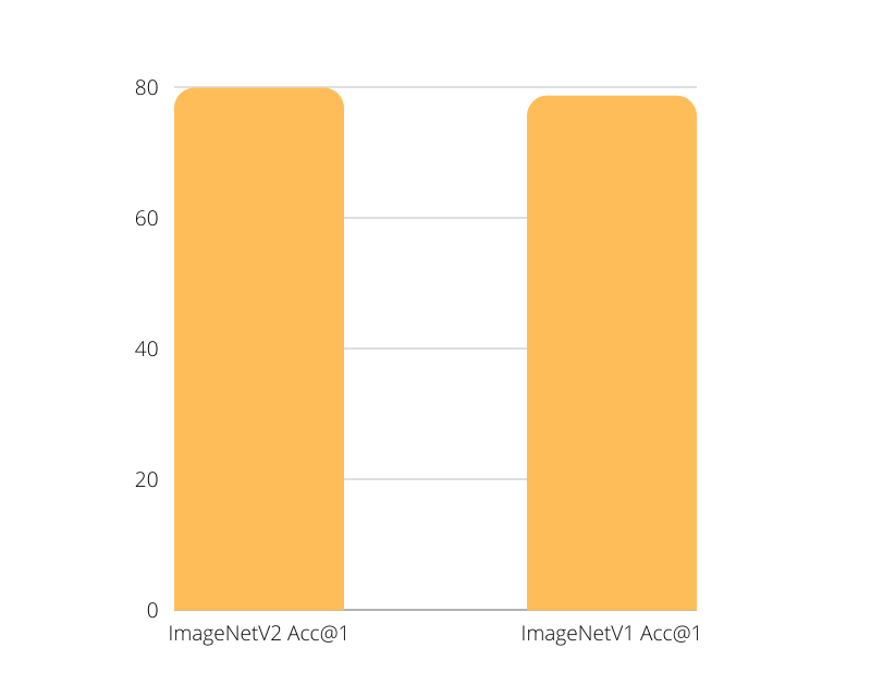
EfficientNetB1 is one of them. The older ImageNet1K_V1 weights give a top-1 accuracy of 78.642% and the new weights give a top-1 accuracy of 79.838%. We have more than a 1% increase in accuracy with the new weights. and most probably, this will be reflected in transfer learning tasks as well.

For the dataset, we are choosing the CIFAR10 dataset. This is because it is not always that easy to get state-of-the-art accuracy on the CIFAR10 dataset when training from scratch. Transfer learning helps a lot and the new ImageNet1K_V2 weights are bound to help in this case.

Installing The Latest Version of PyTorch and Torchvision

To run the code successfully in this blog post, you will need at least PyTorch version 1.12.0 and Torchvision version 0.13.0.

At the time of you reading this, if newer versions have been released, you can install them as well. Install/update PyTorch from here.

Choose either Conda or Pip installation according to your hardware configuration.

Directory Structure

Now, coming to the directory structure. The following block shows the project directory structure for the code files.

├── data
│   ├── cifar-10-batches-py
│   └── cifar-10-python.tar.gz
├── outputs
│   ├── IMAGENET1K_V1_accuracy.png
│   ├── IMAGENET1K_V1_loss.png
│   ├── IMAGENET1K_V1_model.pth
│   ├── IMAGENET1K_V2_accuracy.png
│   ├── IMAGENET1K_V2_loss.png
│   └── IMAGENET1K_V2_model.pth
└── src
    ├── dataset.py
    ├── model.py
    ├── train.py
    └── utils.py

• The data directory contains the CIFAR10 dataset that we will directly download using the torchvision.datasets module.
• The outputs directory contains the loss & accuracy graphs that are generated during the training process. As we will be carrying out two training experiments, one with ImageNet1K_V1 weights and the other with ImageNet1K_V2 weights, so, the files in this directory have a corresponding naming convention.
• All the Python code files are present in the src directory. We will discuss all the details in the coding section.

All the Python code files will be available with the downloadable zip file. You can right away execute the code by directly downloading and extracting the zip file which is already structured as shown above.

Comparing PyTorch ImageNetV1 and ImageNetV2 Weights in Transfer Learning Task

Before jumping into the code, let’s outline the experiments that we will carry out here.

• The first experiment will use the older ImageNet weights for transfer learning. Those are the IMAGENET1K_V1 weights.
• The next experiment will use the new IMAGENET1K_V2 weights.

We will discuss all the dataset preparation and hyperparameter details in the respective sections. Also, we will take a look at how to load both of the ImageNet pretrained weights while preparing the model in model.py.

All the Python files will reside in the src directory.

Download Code

Helper Functions and Utility Code

We will need some helper functions to save the trained model and the loss & accuracy graphs after the training completes.

For that, we will write two simple helper functions in the utils.py file.

import torch
import matplotlib
import matplotlib.pyplot as plt
import os

matplotlib.style.use('ggplot')

def save_model(epochs, model, optimizer, criterion, weights):
    """
    Function to save the trained model to disk.
    """
    torch.save({
                'epoch': epochs,
                'model_state_dict': model.state_dict(),
                'optimizer_state_dict': optimizer.state_dict(),
                'loss': criterion,
                }, os.path.join('..', 'outputs', weights+'_model.pth'))

def save_plots(train_acc, valid_acc, train_loss, valid_loss, weights):
    """
    Function to save the loss and accuracy plots to disk.
    """
    # Accuracy plots.
    plt.figure(figsize=(10, 7))
    plt.plot(
        train_acc, color='tab:blue', linestyle='-', 
        label='train accuracy'
    )
    plt.plot(
        valid_acc, color='tab:red', linestyle='-', 
        label='validataion accuracy'
    )
    plt.xlabel('Epochs')
    plt.ylabel('Accuracy')
    plt.legend()
    plt.savefig(os.path.join('..', 'outputs', weights+'_accuracy.png'))
    
    # Loss plots.
    plt.figure(figsize=(10, 7))
    plt.plot(
        train_loss, color='tab:blue', linestyle='-', 
        label='train loss'
    )
    plt.plot(
        valid_loss, color='tab:red', linestyle='-', 
        label='validataion loss'
    )
    plt.xlabel('Epochs')
    plt.ylabel('Loss')
    plt.legend()
    plt.savefig(os.path.join('..', 'outputs', weights+'_loss.png'))

Both, the save_model and save_plots functions accept a weights parameter which is a string. This specifies whether the weights used for training are the older or newer ImageNet weights. We append this string at the end of the model name and plots to distinguish them. We can also see this in the outputs directory files in the directory structure section.

Next, we have a simple class for the learning rate scheduler. This acts as a simple wrapper around the ReduceLROnPlateau from PyTorch.

class LRScheduler():
    """
    Learning rate scheduler. If the validation loss does not decrease for the 
    given number of `patience` epochs, then the learning rate will decrease by
    by given `factor`.
    """
    def __init__(
        self, optimizer, patience=5, min_lr=1e-6, factor=0.1
    ):
        """
        new_lr = old_lr * factor

        :param optimizer: the optimizer we are using
        :param patience: how many epochs to wait before updating the lr
        :param min_lr: least lr value to reduce to while updating
        :param factor: factor by which the lr should be updated
        """
        self.optimizer = optimizer
        self.patience = patience
        self.min_lr = min_lr
        self.factor = factor

        self.lr_scheduler = torch.optim.lr_scheduler.ReduceLROnPlateau( 
                self.optimizer,
                mode='min',
                patience=self.patience,
                factor=self.factor,
                min_lr=self.min_lr,
                verbose=True
            )

    def __call__(self, val_loss):
        self.lr_scheduler.step(val_loss)

The above class will ensure to reduce the learning rate whenever the validation loss does not improve during training.

This is all we need for the helper code.

Preparing the CIFAR10 Data

Although the CIFAR10 data is directly available in the torchvision.datasets module, we will write some simple and additional code here.

All the code for dataset preparation will go into the dataset.py file.

First, we we have the import statements and the functions defining transforms and augmentations.

import os

from torchvision import datasets, transforms
from torch.utils.data import DataLoader

# Image size.
IMAGE_SIZE = 64 # Image size of resize when applying transforms.

# Training transforms
def get_train_transform(image_size):
    train_transform = transforms.Compose([
        transforms.Resize((image_size, image_size)),
        transforms.RandomRotation(30),
        transforms.RandomAdjustSharpness(sharpness_factor=2, p=0.5),
        transforms.RandomAutocontrast(p=0.5),
        transforms.ToTensor(),
        transforms.Normalize(
            mean=[0.485, 0.456, 0.406],
            std=[0.229, 0.224, 0.225]
            )
    ])
    return train_transform

# Validation transforms
def get_valid_transform(image_size):
    valid_transform = transforms.Compose([
        transforms.Resize((image_size, image_size)),
        transforms.ToTensor(),
        transforms.Normalize(
            mean=[0.485, 0.456, 0.406],
            std=[0.229, 0.224, 0.225]
            )
    ])
    return valid_transform

The get_train_transform function contains a few augmentations. These will ensure that the powerful EfficientNetB1 model does not easily overfit on the CIFAR10 dataset. Apart from that, we resize all the images to 64×64 resolution, convert them to tensors, and apply the ImageNet normalization stats.

We do almost the same thing in the validation transforms apart from the augmentations.

Next, we have two functions, one to prepare the dataset, and the other for the data loaders.

def get_datasets():
    """
    Function to prepare the Datasets.
    Returns the training and validation datasets along 
    with the class names.
    """
    dataset_train = datasets.CIFAR10(
        root=os.path.join('..', 'data'), 
        train=True,
        download=True, 
        transform=get_train_transform(IMAGE_SIZE)
    )
    dataset_valid = datasets.CIFAR10(
        root=os.path.join('..', 'data'), 
        train=False,
        download=True, 
        transform=get_valid_transform(IMAGE_SIZE)
    )
    return dataset_train, dataset_valid, dataset_train.classes

def get_data_loaders(
    dataset_train, 
    dataset_valid, 
    train_batch_size,
    valid_batch_size, 
    num_workers
):
    """
    Prepares the training and validation data loaders.
    :param dataset_train: The training dataset.
    :param dataset_valid: The validation dataset.
    Returns the training and validation data loaders.
    """
    train_loader = DataLoader(
        dataset_train, batch_size=train_batch_size, 
        shuffle=True, num_workers=num_workers
    )
    valid_loader = DataLoader(
        dataset_valid, batch_size=valid_batch_size, 
        shuffle=False, num_workers=num_workers
    )
    return train_loader, valid_loader 

The get_datasets prepares the training and validation dataset. It returns the corresponding datasets along with the class names.

The get_data_loaders function accepts the datasets, batch sizes, and the number of workers as parameters. It simply creates the data loaders and returns them.

All the code for CIFAR10 dataset preparation is complete with this.

The EfficientNetB1 Model for Loading PyTorch ImageNetV1 and ImageNetV2 Weights

Let’s get down to the most important part of the post. Preparing the EfficientNetB1 model. This is perhaps the easiest part of the entire experiment as well.

The code for the model preparation will go into the model.py file.

The following block contains the entire code.

import torchvision.models as models
import torch.nn as nn

def build_model(
    weights='IMAGENET1K_V2', 
    fine_tune=False, 
    num_classes=10
):
    if weights:
        print(f"[INFO]: Loading {weights} pre-trained weights")
    else:
        print('[INFO]: Not loading pre-trained weights')
    model = models.efficientnet_b1(weights=weights)

    if fine_tune:
        print('[INFO]: Fine-tuning all layers...')
        for params in model.parameters():
            params.requires_grad = True
    elif not fine_tune:
        print('[INFO]: Freezing hidden layers...')
        for params in model.parameters():
            params.requires_grad = False

    # Change the final classification head.
    model.classifier[1] = nn.Linear(in_features=1280, out_features=num_classes)
    return model

The build_model function accepts three parameters:

• weights: Instead of the older pretrained argument, we now have to use the weights argument while loading the model. And we cannot just specify True or False anymore. We need to specify which ImageNet weights we want to use. Either IMAGENET1K_V1 or IMAGENET1K_V2.
• fine_tune: This will control whether we want to train the entire model or not.
• num_classes: To specify the number of classes for the final output layer.

Do observe that on line 13, we are using the string value passed to the weights parameter in the function definition. This is one of the simpler ways to control whether we want to load the older or newer ImageNet weights. There are other ways also, which you can find here.

Then we specify whether to fine-tune all layers or not and change the number of output features in the final Linear layer.

The Training Script for Comparing PyTorch ImageNetV1 and ImageNetV2 Weights

Let’s get down to the training script now. This is where we combine everything that we have been writing till now.

The train.py file is an executable script that contains the final training code.

First, let’s import all the libraries and modules that we need, prepare the argument parser, and set the seed for reproducibility.

import torch
import argparse
import torch.nn as nn
import torch.optim as optim
import time

from tqdm.auto import tqdm
from model import build_model
from dataset import get_datasets, get_data_loaders
from utils import save_model, save_plots, LRScheduler

# Construct the argument parser.
parser = argparse.ArgumentParser()
parser.add_argument(
    '-e', '--epochs', type=int, default=20,
    help='number of epochs to train our network for'
)
parser.add_argument(
    '-b', '--batch-size', dest='batch_size', type=int, default=16,
    help='batch size for data loaders'
)
parser.add_argument(
    '-lr', '--learning-rate', type=float,
    dest='learning_rate', default=0.001,
    help='learning rate for training the model'
)
parser.add_argument(
    '-w', '--weights', type=str, default='IMAGENET1K_V2',
    help='ImageNet weight to use [IMAGENET1K_V1, IMAGENET1K_V2]',
    choices=['IMAGENET1K_V1', 'IMAGENET1K_V2']
)
args = vars(parser.parse_args())

# Set seed.
seed = 42
torch.manual_seed(seed)
torch.cuda.manual_seed(seed)
torch.backends.cudnn.deterministic = True
torch.backends.cudnn.benchmark = True

Among the modules, we also have our custom ones like model, dataset, and utils.

For the argument parsers, we have:

• --epochs: Flag to control the number of epochs to train for.
• --batch-size: Flag to set the batch size for the data loaders.
• --learning-rate: To set the learning rate when starting the training. This is helpful when trying out different optimizers or switching between training from scratch and transfer learning.
• --weights: The pretrained weights to use. We can either provide IMAGENET1K_V1 or IMAGENET1K_V2.

Then we set all the possible seeds for torch to get the same values across multiple runs.

The Training and Validation Functions

We will use very simple training and validation functions that are almost common everywhere for image classification in PyTorch.

The following code block contains the training function.

# Training function.
def train(model, trainloader, optimizer, criterion):
    model.train()
    print('Training')
    train_running_loss = 0.0
    train_running_correct = 0
    counter = 0
    for i, data in tqdm(enumerate(trainloader), total=len(trainloader)):
        counter += 1
        image, labels = data
        image = image.to(device)
        labels = labels.to(device)
        optimizer.zero_grad()
        # Forward pass.
        outputs = model(image)
        # Calculate the loss.
        loss = criterion(outputs, labels)
        train_running_loss += loss.item()
        # Calculate the accuracy.
        _, preds = torch.max(outputs.data, 1)
        train_running_correct += (preds == labels).sum().item()
        # Backpropagation
        loss.backward()
        # Update the weights.
        optimizer.step()
    
    # Loss and accuracy for the complete epoch.
    epoch_loss = train_running_loss / counter
    # epoch_acc = 100. * (train_running_correct / len(trainloader.dataset))
    epoch_acc = 100. * (train_running_correct / len(trainloader.dataset))
    return epoch_loss, epoch_acc

In the training loop, we get the outputs by forward passing the images through the model, then calculate the loss, do the backpropagation, and return the loss & accuracy value for each epoch.

Next is the validation function.

# Validation function.
def validate(model, testloader, criterion):
    model.eval()
    print('Validation')
    valid_running_loss = 0.0
    valid_running_correct = 0
    counter = 0

    with torch.no_grad():
        for i, data in tqdm(enumerate(testloader), total=len(testloader)):
            counter += 1
            
            image, labels = data
            image = image.to(device)
            labels = labels.to(device)
            # Forward pass.
            outputs = model(image)
            # Calculate the loss.
            loss = criterion(outputs, labels)
            valid_running_loss += loss.item()
            # Calculate the accuracy.
            _, preds = torch.max(outputs.data, 1)
            valid_running_correct += (preds == labels).sum().item()
        
    # Loss and accuracy for the complete epoch.
    epoch_loss = valid_running_loss / counter
    epoch_acc = 100. * (valid_running_correct / len(testloader.dataset))
    return epoch_loss, epoch_acc

We do not need any backpropagation or gradient update in the validation loop. Still, we return the validation accuracy and loss value for each epoch.

The Main Block

Finally, we need to write the code for the main block (if __name__=='__main__').

if __name__ == '__main__':
    # Load the training and validation datasets.
    dataset_train, dataset_valid, classes = get_datasets()
    print(f"[INFO]: Number of training images: {len(dataset_train)}")
    print(f"[INFO]: Number of validation images: {len(dataset_valid)}")
    print(f"[INFO]: Classes: {classes}")
    # Load the training and validation data loaders.
    train_loader, valid_loader = get_data_loaders(
        dataset_train=dataset_train, 
        dataset_valid=dataset_valid,
        train_batch_size=args['batch_size'],
        valid_batch_size=args['batch_size'],
        num_workers=4
    )

    # Learning_parameters. 
    lr = args['learning_rate']
    epochs = args['epochs']
    device = ('cuda' if torch.cuda.is_available() else 'cpu')
    print(f"Computation device: {device}")
    print(f"Learning rate: {lr}")
    print(f"Epochs to train for: {epochs}\n")

    # Load the model.
    model = build_model(
        weights=args['weights'],
        fine_tune=True, 
        num_classes=len(classes)
    ).to(device)
    
    # Total parameters and trainable parameters.
    total_params = sum(p.numel() for p in model.parameters())
    print(f"{total_params:,} total parameters.")
    total_trainable_params = sum(
        p.numel() for p in model.parameters() if p.requires_grad)
    print(f"{total_trainable_params:,} training parameters.")

    # Optimizer.
    optimizer = optim.Adam(model.parameters(), lr=lr)
    # Loss function.
    criterion = nn.CrossEntropyLoss()
    # Initialize LR scheduler.
    lr_scheduler = LRScheduler(optimizer, patience=1, factor=0.5)

    # Lists to keep track of losses and accuracies.
    train_loss, valid_loss = [], []
    train_acc, valid_acc = [], []
    # Start the training.
    for epoch in range(epochs):
        print(f"[INFO]: Epoch {epoch+1} of {epochs}")
        train_epoch_loss, train_epoch_acc = train(
            model, 
            train_loader, 
            optimizer, 
            criterion
        )
        valid_epoch_loss, valid_epoch_acc = validate(
            model, 
            valid_loader, 
            criterion
        )
        train_loss.append(train_epoch_loss)
        valid_loss.append(valid_epoch_loss)
        train_acc.append(train_epoch_acc)
        valid_acc.append(valid_epoch_acc)
        print(f"Training loss: {train_epoch_loss:.3f}, training acc: {train_epoch_acc:.3f}")
        print(f"Validation loss: {valid_epoch_loss:.3f}, validation acc: {valid_epoch_acc:.3f}")
        lr_scheduler(valid_epoch_loss)
        print('-'*50)
        time.sleep(5)
        
    # Save the trained model weights.
    save_model(epochs, model, optimizer, criterion, args['weights'])
    # Save the loss and accuracy plots.
    save_plots(train_acc, valid_acc, train_loss, valid_loss, args['weights'])
    print('TRAINING COMPLETE')

The following points highlight the important bits from the above code block.

• We prepare the datasets and data loaders on lines 101 and 106 respectively.
• The model initialization happens on line 123. Here we pass the weights name from the argument parser to the weights argument, so as to load the corresponding weights. We do not have to hardcode anything.
• Then we define the optimizer and the loss function and initialize the learning rate scheduler as well. Note that the patience is set to 1 and each time the learning rate will be reduced by half.
• Then starting from line 147, we have the training and validation loops. We have the loss and accuracy values in their respective lists which we use in the end for plotting the graphs. We also save the models after the training completes.

This completes all the code that we need for comparing the PyTorch ImageNetV1 and ImageNetV2 weights for transfer learning tasks. Let’s execute the training script to carry out the experiments now.

Executing train.py

Note that the training experiments have been carried out on a machine with 10 GB RTX 3080 GPU, i7 10th generation CPU, and 32 GB of RAM. Your training time may vary depending on the hardware.

As discussed earlier, we will be executing the train.py twice. Once with ImageNetV1 weights for the EfficientNetB1 model, and again with the ImageNetV2 weights.

IMAGENET1K_V1 Training

Beginning with the IMAGENET1K_V1 weights. Be sure to execute the train.py script within the src directory.

python train.py --epochs 25 --weights IMAGENET1K_V1 --batch-size 128 --learning-rate 0.0001

We are training for 25 epochs here. Notice that the weights are set to IMAGENET1K_V1. The batch size is set to 128. If you get run out of GPU memory (OOM error), please reduce the batch size to either 64 or 32. As we are using pretrained weights here, so the initial learning rate is set to 0.0001.

The following block shows the truncated outputs for the above training.

Files already downloaded and verified
Files already downloaded and verified
[INFO]: Number of training images: 50000
[INFO]: Number of validation images: 10000
[INFO]: Classes: ['airplane', 'automobile', 'bird', 'cat', 'deer', 'dog', 'frog', 'horse', 'ship', 'truck']
Computation device: cuda
Learning rate: 0.0001
Epochs to train for: 25

[INFO]: Loading IMAGENET1K_V1 pre-trained weights
[INFO]: Fine-tuning all layers...
6,525,994 total parameters.
6,525,994 training parameters.
[INFO]: Epoch 1 of 25
Training
100%|██████████████████████████████████████████████████████████████████| 391/391 [00:36<00:00, 10.64it/s]
Validation
100%|████████████████████████████████████████████████████████████████████| 79/79 [00:01<00:00, 67.79it/s]
Training loss: 1.482, training acc: 48.324
Validation loss: 0.823, validation acc: 72.590
--------------------------------------------------
[INFO]: Epoch 2 of 25
Training
100%|██████████████████████████████████████████████████████████████████| 391/391 [00:33<00:00, 11.74it/s]
Validation
100%|████████████████████████████████████████████████████████████████████| 79/79 [00:01<00:00, 76.80it/s]
Training loss: 0.768, training acc: 73.416
Validation loss: 0.538, validation acc: 81.620
--------------------------------------------------
.
.
.
[INFO]: Epoch 24 of 25
Training
100%|██████████████████████████████████████████████████████████████████| 391/391 [00:35<00:00, 11.03it/s]
Validation
100%|████████████████████████████████████████████████████████████████████| 79/79 [00:01<00:00, 45.76it/s]
Training loss: 0.088, training acc: 97.000
Validation loss: 0.285, validation acc: 91.670
Epoch 00024: reducing learning rate of group 0 to 1.0000e-06.
--------------------------------------------------
[INFO]: Epoch 25 of 25
Training
100%|██████████████████████████████████████████████████████████████████| 391/391 [00:35<00:00, 11.02it/s]
Validation
100%|████████████████████████████████████████████████████████████████████| 79/79 [00:01<00:00, 47.79it/s]
Training loss: 0.086, training acc: 97.084
Validation loss: 0.287, validation acc: 91.390
--------------------------------------------------
TRAINING COMPLETE

By the end of 25 epochs, we have a validation accuracy of 91.39%. This looks pretty good considering that we did not do anything fancy. But right now, we don’t have anything to compare this value with. Still, let’s take a look at the accuracy and loss graphs.

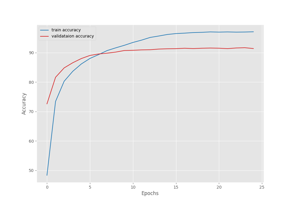
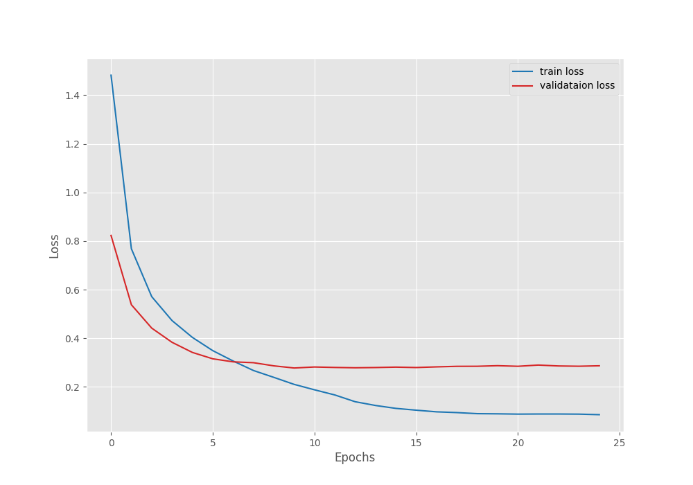
It seems that due to the learning rate scheduler, both, the validation accuracy and loss seem to plateau out by the end of training. But maybe, if we do not reduce them as aggressively as now, there is a chance of overfitting.

IMAGENET1K_V2 Training

Now, executing the training script with the IMAGENET1K_V2 weights.

python train.py --epochs 25 --weights IMAGENET1K_V2 --batch-size 128 --learning-rate 0.0001

This time, we just change the value for the --weights flag.

Files already downloaded and verified
Files already downloaded and verified
[INFO]: Number of training images: 50000
[INFO]: Number of validation images: 10000
[INFO]: Classes: ['airplane', 'automobile', 'bird', 'cat', 'deer', 'dog', 'frog', 'horse', 'ship', 'truck']
Computation device: cuda
Learning rate: 0.0001
Epochs to train for: 25

[INFO]: Loading IMAGENET1K_V2 pre-trained weights
[INFO]: Fine-tuning all layers...
6,525,994 total parameters.
6,525,994 training parameters.
[INFO]: Epoch 1 of 25
Training
100%|██████████████████████████████████████████████████████████████████| 391/391 [00:35<00:00, 11.10it/s]
Validation
100%|████████████████████████████████████████████████████████████████████| 79/79 [00:02<00:00, 35.28it/s]
Training loss: 1.265, training acc: 57.120
Validation loss: 0.565, validation acc: 80.720
--------------------------------------------------
[INFO]: Epoch 2 of 25
Training
100%|██████████████████████████████████████████████████████████████████| 391/391 [00:32<00:00, 11.96it/s]
Validation
100%|████████████████████████████████████████████████████████████████████| 79/79 [00:01<00:00, 39.87it/s]
Training loss: 0.621, training acc: 78.504
Validation loss: 0.423, validation acc: 85.530
--------------------------------------------------
.
.
.
[INFO]: Epoch 24 of 25
Training
100%|██████████████████████████████████████████████████████████████████| 391/391 [00:35<00:00, 10.94it/s]
Validation
100%|████████████████████████████████████████████████████████████████████| 79/79 [00:01<00:00, 62.76it/s]
Training loss: 0.081, training acc: 97.154
Validation loss: 0.254, validation acc: 92.610
Epoch 00024: reducing learning rate of group 0 to 3.1250e-06.
--------------------------------------------------
[INFO]: Epoch 25 of 25
Training
100%|██████████████████████████████████████████████████████████████████| 391/391 [00:35<00:00, 10.94it/s]
Validation
100%|████████████████████████████████████████████████████████████████████| 79/79 [00:01<00:00, 63.61it/s]
Training loss: 0.077, training acc: 97.316
Validation loss: 0.255, validation acc: 92.480
--------------------------------------------------
TRAINING COMPLETE

We have higher a validation accuracy of 92.48% this time. The validation loss is also lower compared to the previous training. In fact, the increase in accuracy almost matches the just over 1% increase for the actual pretrained weights for ImageNetV2 weights. Most likely a coincidence, or maybe not.

This time also, the validation plots seem to be following a similar trend of plateauing out by the end of the training.

From the above experiments, we can conclude that the new ImageNet pretrained weights offer a slight advantage over the older weights. And most probably, a more comprehensive experiment will be needed across different models and a better real-world dataset other than CIFAR10 to conclude anything concretely. If you happen to carry experiments for other models, be sure to tell about the results in the comment section.

Summary and Conclusion

In this blog post, we carried out a very simple experiment for comparing the ImageNetV1 and ImageNetV2 pretrained weights in PyTorch. Even with a simple dataset like CIFAR10, we were able to get a higher validation accuracy with the new ImageNet weights. So, there seems to be an improvement in the transfer learning task. I hope that this blog post helped you in learning something new.

If you have any doubts, thoughts, or suggestions, please leave them in the comment section. I will surely address them.

You can contact me using the Contact section. You can also find me on LinkedIn, and Twitter.