A Detailed Comparison Between PyTorch IMAGENET1K_V1 and IMAGENET1K_V2 Weights

With the release of PyTorch 1.12.0, some models now have a new set of ImageNet pretrained weights, the IMAGENET1K_V2 weights. As such, the older weights for these particular models are known as the IMAGENET1K_V1 weights. Essentially, the vision (Torchvision 0.13.0) library received these updates. And as per the claim, the newer weights appear to provide 3% higher accuracy in some cases. In this post, we will do a detailed comparison between the PyTorch IMAGENET1K_V1 and IMAGENET1K_V2 weights in transfer learning and fine-tuning. This will give us a proper idea on the kind of improvements to expect when using the newer weights.

In the last post, we saw that indeed the EfficientNetB1 IMAGENET1K_V2 weights provided a higher accuracy when fine-tuning on the CIFAR10 dataset. But CIFAR10 may not be a good dataset for such an experiment. We may need a dataset resembling images from real life. Also, only fine-tuning (training all layers) may not be an appropriate check. We should also check out transfer learning (freezing the intermediate layers). We will do all these experiments in this post using the ResNet50 model and the Intel Image Classification Dataset.

We will cover the following topics in this post:

• We will start with the discussion of the Intel Image Classification Dataset from Kaggle.
• Then we will discuss briefly the ResNet50 IMAGENET1K_V2 weights.
• Here, we will carry out 4 different experiments:
  • Transfer learning using IMAGENET1K_V1 weights.
  • Transfer learning using IMAGENET1K_V2 weights.
  • Fine-tuning using the IMAGENET1K_V1 weights.
  • Fine-tuning using the IMAGENET1K_V2 weights.

These four experiments should give us a good idea of whether we can expect an increase in accuracy when using the new ImageNet pretrained weights. And if so, to what extent.

The Intel Image Classification Dataset

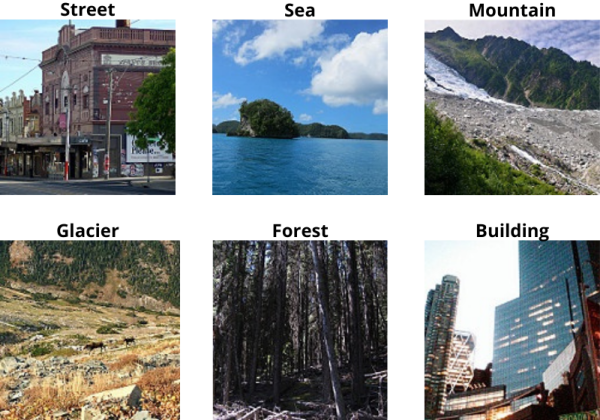
We will use the Intel Image Classification dataset from Kaggle for the experiments in this post. The main reason for this dataset is that the images resemble a real-world set. It contains images of natural scenes from around the world. All images belong to one of the following 6 classes:

• Building – Class 0.
• Forest – Class 1.
• Glacier – Class 2.
• Mountain – Class 3.
• Sea – Class 4.
• Street – Class 5.

After downloading and extracting the dataset, we find it in the following directory structure.

├── seg_pred
│   └── seg_pred [7301 entries exceeds filelimit, not opening dir]
├── seg_test
│   └── seg_test
│       ├── buildings [437 entries exceeds filelimit, not opening dir]
│       ├── forest [474 entries exceeds filelimit, not opening dir]
│       ├── glacier [553 entries exceeds filelimit, not opening dir]
│       ├── mountain [525 entries exceeds filelimit, not opening dir]
│       ├── sea [510 entries exceeds filelimit, not opening dir]
│       └── street [501 entries exceeds filelimit, not opening dir]
└── seg_train
    └── seg_train
        ├── buildings [2191 entries exceeds filelimit, not opening dir]
        ├── forest [2271 entries exceeds filelimit, not opening dir]
        ├── glacier [2404 entries exceeds filelimit, not opening dir]
        ├── mountain [2512 entries exceeds filelimit, not opening dir]
        ├── sea [2274 entries exceeds filelimit, not opening dir]
        └── street [2382 entries exceeds filelimit, not opening dir]

We have three directories.

• The seg_train directory contains all the images for training inside the respective class directories. There are over 14000 images in the training set. We will use these images in the training loop while training the ResNet50 model.
• The seg_test directory contains the test images in a similar way. All the images are in their respective class directories. There are around 3000 images for testing and we will use these in the validation loop while training the model.
• We also have a seg_pred directory without any class subdirectories. These are mainly for inference but we will not need these in this blog post. Although one may run inference on these after the model trains. However, as no ground-truth data is available for these, one has to evaluate each of them manually.

All the images are 150×150 resolution RGB images. For now, you can go ahead and download the dataset. In one of the later sections, we will check out how to structure the entire project directory along with the dataset.

The ResNet50 IMAGENET1K_V2 Weights

Let’s briefly check out the ResNet IMAGENET1K_V2 weights.

We can find all details about the ResNet50 weights, both old and new, here. This official documentation contains all the information on the IMAGENET1K_V1 and IMAGENET1K_V2 weights. Going over the tables shows that the new ImageNet weights give a top-1 accuracy of 80.858%. This is more than a 4.7% increase from the older 76.13%. Even the top-5 accuracy is ahead by more than 2.5% with new ImageNet weights.

And note that this is while keeping the architecture the same. This means that the number of parameters remains the same. Yet such a huge improvement in accuracy. And surely, this is going to help in transfer learning and fine-tuning tasks.

Experiments To Carry Out for Comparison Between PyTorch IMAGENET1K_V1 and IMAGENET1K_V2 Weights

In this blog post, we will carry out 4 experiments. The following points contain a brief of all those.

• Transfer Learning using IMAGENET1K_V1 Weights:
  • We will begin with transfer learning with the older weights, that is IMAGENET1K_V1 weights. We will freeze all the hidden layers of the ResNet50 model and train the classification head only.
• Transfer Learning using IMAGENET1K_V2 Weights:
  • This is similar to the previous experiment. But we will use the new IMAGENET1K_V2 weights in this experiment.
• Fine-tuning using IMAGENET1K_V1 Weights:
  • We will again use the IMAGENET1K_V1 weights here. But this time, we will fine-tune the entire model instead of training just the classification head.
• Fine-tuning using IMAGENET1K_V2 Weights:
  • Here, again we will train the entire model but using the new IMAGENET1K_V2 weights.

In all of the above experiments, we will apply some minor augmentations to prevent overfitting too soon. We will apply the following augmentations to the training data from torchvision.transforms:

• RandomHorizontalFlip: To randomly flip an image horizontally.
• RandomRotation: To rotate an image randomly by a certain degree.
• RandomAdjustSharpness: For changing the sharpness of an image.

These augmentations will ensure that the models get to see some variability in the images. Also, this will give us an idea of how each of the pretrained weights behaves under different conditions.

Installing The Latest Version of PyTorch and Torchvision

To run the code successfully in this blog post, you will need at least PyTorch version 1.12.0 and Torchvision version 0.13.0.

At the time of you reading this, if newer versions have been released, you can install them as well. Install/update PyTorch from here.

Choose either Conda or Pip installation according to your hardware configuration.

Directory Structure

The following is the directory structure for the code and data in this blog post.

├── input
│   ├── seg_pred
│   │   └── seg_pred [7301 entries exceeds filelimit, not opening dir]
│   ├── seg_test
│   │   └── seg_test
│   │       ├── buildings [437 entries exceeds filelimit, not opening dir]
│   │       ├── forest [474 entries exceeds filelimit, not opening dir]
│   │       ├── glacier [553 entries exceeds filelimit, not opening dir]
│   │       ├── mountain [525 entries exceeds filelimit, not opening dir]
│   │       ├── sea [510 entries exceeds filelimit, not opening dir]
│   │       └── street [501 entries exceeds filelimit, not opening dir]
│   ├── seg_train
│   │   └── seg_train
│   │       ├── buildings [2191 entries exceeds filelimit, not opening dir]
│   │       ├── forest [2271 entries exceeds filelimit, not opening dir]
│   │       ├── glacier [2404 entries exceeds filelimit, not opening dir]
│   │       ├── mountain [2512 entries exceeds filelimit, not opening dir]
│   │       ├── sea [2274 entries exceeds filelimit, not opening dir]
│   │       └── street [2382 entries exceeds filelimit, not opening dir]
│   └── intel-image-classification.zip
├── outputs
│   ├── IMAGENET1K_V1_ftFalse_accuracy.png
│   ...
│   └── IMAGENET1K_V2_ftTrue_model.pth
└── src
    ├── dataset.py
    ├── model.py
    ├── train.py
    └── utils.py

We have already seen the structure of the input directory which contains the dataset. Let’s go over the rest of the directories.

• The outputs directory contains the outputs from all the training experiments. These include the accuracy & loss graphs along with the trained models. Although we will not use the trained models in this blog post anywhere. However, you can choose to use them to run inference over images in the seg_pred directory of the dataset.
• The src directory contains the Python code files. We have four files dealing with all the code in this post.
  • We have the dataset and data loader creation code in the dataset.py file.
  • The model.py file contains the code to load the ResNet50 model along with appropriate parameters and settings.
  • The utils.py contains the helper code to save the plots, the trained model, and code for the learning rate scheduler as well.
  • Finally, the train.py is the executable script which combines all the modules and runs the experiments.

Note: The code is available to download in this post. But we will not cover the code here in the blog post other than that of the neural network model. We will also briefly cover the arguments that we can pass to the train.py script to avoid confusion. Rather, we will entirely focus on the results that we get after running each experiment. Most of them are general PyTorch code which is pretty straightforward and easy to follow.

Comparison Between PyTorch IMAGENET1K_V1 and IMAGENET1K_V2 Weights

In this section, we will dive into the experiments and their results. But before that, let’s take a look at the code for the ResNet50 model. Along with that, we will also check out the command line argument flags for the training script. This will make the experiment section simpler to follow.

Download Code

Beginning with the ResNet50 model code.

import torchvision.models as models
import torch.nn as nn

def build_model(
    weights='IMAGENET1K_V2', 
    fine_tune=False, 
    num_classes=10
):
    if weights:
        print(f"[INFO]: Loading {weights} pre-trained weights")
    else:
        print('[INFO]: Not loading pre-trained weights')
    model = models.resnet50(weights=weights)

    if fine_tune:
        print('[INFO]: Fine-tuning all layers...')
        for params in model.parameters():
            params.requires_grad = True
    elif not fine_tune:
        print('[INFO]: Freezing hidden layers...')
        for params in model.parameters():
            params.requires_grad = False

    # Change the final classification head.
    model.fc = nn.Linear(in_features=2048, out_features=num_classes)
    return model

The build_model function accepts three parameters:

• weights: This is a string specifying which ImageNet weight to use. We can either pass IMAGENET1K_V1 or IMAGENET1K_V2 as an argument for this. This string is again used on line 13 to load the specific ImageNet pretrained weight.
• fine_tune: This is a boolean value. If it is True, all the layers are trainable, else only the classification head is trainable.
• num_classes: The number of classes for the output features in the final classification head.

Next, let’s check out all the command line flags that we can use while executing train.py.

#...
# Construct the argument parser.
parser = argparse.ArgumentParser()
parser.add_argument(
    '-e', '--epochs', type=int, default=20,
    help='number of epochs to train our network for'
)
parser.add_argument(
    '-b', '--batch-size', dest='batch_size', type=int, default=16,
    help='batch size for data loaders'
)
parser.add_argument(
    '-lr', '--learning-rate', type=float,
    dest='learning_rate', default=0.001,
    help='learning rate for training the model'
)
parser.add_argument(
    '-w', '--weights', type=str, default='IMAGENET1K_V2',
    help='ImageNet weight to use [IMAGENET1K_V1, IMAGENET1K_V2]',
    choices=['IMAGENET1K_V1', 'IMAGENET1K_V2']
)
parser.add_argument(
    '-ft', '--fine-tune', action='store_true',
    help='whether to fine tune all layers or not'
)
args = vars(parser.parse_args())
#...

• --epochs: The number of epochs to train for.
• --batch-size: The batch size to use for the training and validation data loaders.
• --learning-rate: As we are using pretrained weights, controlling the learning rate while executing the script is much easier than hard-coding it.
• --weights: The ImageNet weights to use. We can pass either IMAGENET1K_V1 or IMAGENET1K_V2.
• --fine-tune: This is a boolean flag specifying whether we want to fine-tune all the layers of the model or not.

This is all we need to know before executing the training script and diving into the actual experiments.

Experiment for Transfer Learning using IMAGENET1K_V1 Weights

Note: All training experiments for comparison between PyTorch IMAGENET1K_V1 and IMAGENET1K_V2 weights were run on a machine with 10 GB RTX 3080 GPU, 10th generation i7 CPU, and 32 GB of RAM.

We will begin with the fine-tuning experiment using the IMAGENET1K_V1 weights. Here, we will freeze all the intermediate layers of the ResNet50 model and train the final classification head only.

If you want to carry out the experiments, you may also execute the following scripts from the terminal within the src directory.

python train.py --epochs 10 --weights IMAGENET1K_V1 --batch-size 64 --learning-rate 0.0005

We are training for 10 epochs with a batch size of 64. The learning rate is 0.0005, which is lower than the default (0.001 for Adam) as we are loading the pretrained weights.

The following block shows the truncated outputs.

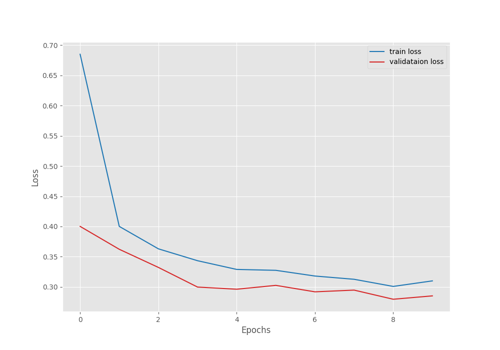
[INFO]: Number of training images: 14034
[INFO]: Number of validation images: 3000
[INFO]: Classes: ['buildings', 'forest', 'glacier', 'mountain', 'sea', 'street']
Computation device: cuda
Learning rate: 0.0005
Epochs to train for: 10

[INFO]: Loading IMAGENET1K_V1 pre-trained weights
[INFO]: Freezing hidden layers...
23,520,326 total parameters.
12,294 training parameters.
[INFO]: Epoch 1 of 10
Training
100%|██████████████████████████████████████████████████████████████████| 220/220 [00:16<00:00, 13.04it/s]
Validation
100%|████████████████████████████████████████████████████████████████████| 47/47 [00:03<00:00, 14.26it/s]
Training loss: 0.685, training acc: 79.307
Validation loss: 0.400, validation acc: 87.933
--------------------------------------------------
[INFO]: Epoch 2 of 10
Training
100%|██████████████████████████████████████████████████████████████████| 220/220 [00:14<00:00, 15.15it/s]
Validation
100%|████████████████████████████████████████████████████████████████████| 47/47 [00:03<00:00, 15.38it/s]
Training loss: 0.400, training acc: 86.711
Validation loss: 0.362, validation acc: 87.600
-------------------------------------------------- 
.
.
.
[INFO]: Epoch 10 of 10
Training
100%|██████████████████████████████████████████████████████████████████| 220/220 [00:14<00:00, 15.02it/s]
Validation
100%|████████████████████████████████████████████████████████████████████| 47/47 [00:02<00:00, 15.82it/s]
Training loss: 0.310, training acc: 88.898
Validation loss: 0.285, validation acc: 89.267
--------------------------------------------------
TRAINING COMPLETE

By the end of the training, we have a validation accuracy of 89.26% and a validation loss of 0.285.

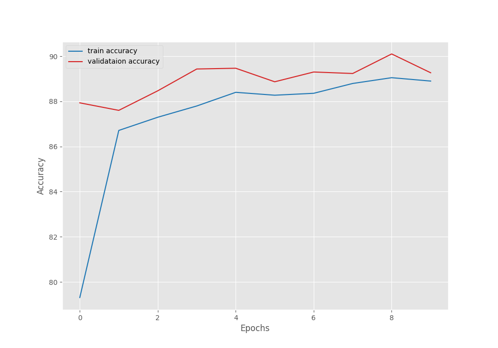
The accuracy seems good considering we trained only the classification head. But most probably, we will get a higher accuracy when we train using the IMAGENET1K_V2 weights.

Transfer Learning using IMAGENET1K_V2 Weights

Here, except the --weights flag, all other flags remain the same as in the previous experiment.

python train.py --epochs 10 --weights IMAGENET1K_V2 --batch-size 64 --learning-rate 0.0005

Let’s check out the results.

[INFO]: Number of training images: 14034
[INFO]: Number of validation images: 3000
[INFO]: Classes: ['buildings', 'forest', 'glacier', 'mountain', 'sea', 'street']
Computation device: cuda
Learning rate: 0.0005
Epochs to train for: 10

[INFO]: Loading IMAGENET1K_V2 pre-trained weights
[INFO]: Freezing hidden layers...
23,520,326 total parameters.
12,294 training parameters.
[INFO]: Epoch 1 of 10
Training
100%|██████████████████████████████████████████████████████████████████| 220/220 [00:16<00:00, 12.99it/s]
Validation
100%|████████████████████████████████████████████████████████████████████| 47/47 [00:03<00:00, 13.78it/s]
Training loss: 0.750, training acc: 81.189
Validation loss: 0.458, validation acc: 87.300
--------------------------------------------------
[INFO]: Epoch 2 of 10
Training
100%|██████████████████████████████████████████████████████████████████| 220/220 [00:15<00:00, 14.55it/s]
Validation
100%|████████████████████████████████████████████████████████████████████| 47/47 [00:02<00:00, 15.67it/s]
Training loss: 0.409, training acc: 87.723
Validation loss: 0.377, validation acc: 88.167
--------------------------------------------------
.
.
.
[INFO]: Epoch 10 of 10
Training
100%|██████████████████████████████████████████████████████████████████| 220/220 [00:14<00:00, 14.85it/s]
Validation
100%|████████████████████████████████████████████████████████████████████| 47/47 [00:02<00:00, 16.07it/s]
Training loss: 0.257, training acc: 91.157
Validation loss: 0.262, validation acc: 90.867
--------------------------------------------------
TRAINING COMPLETE

This time we get more than a 1% increase in the validation accuracy. The validation loss is lower as well.

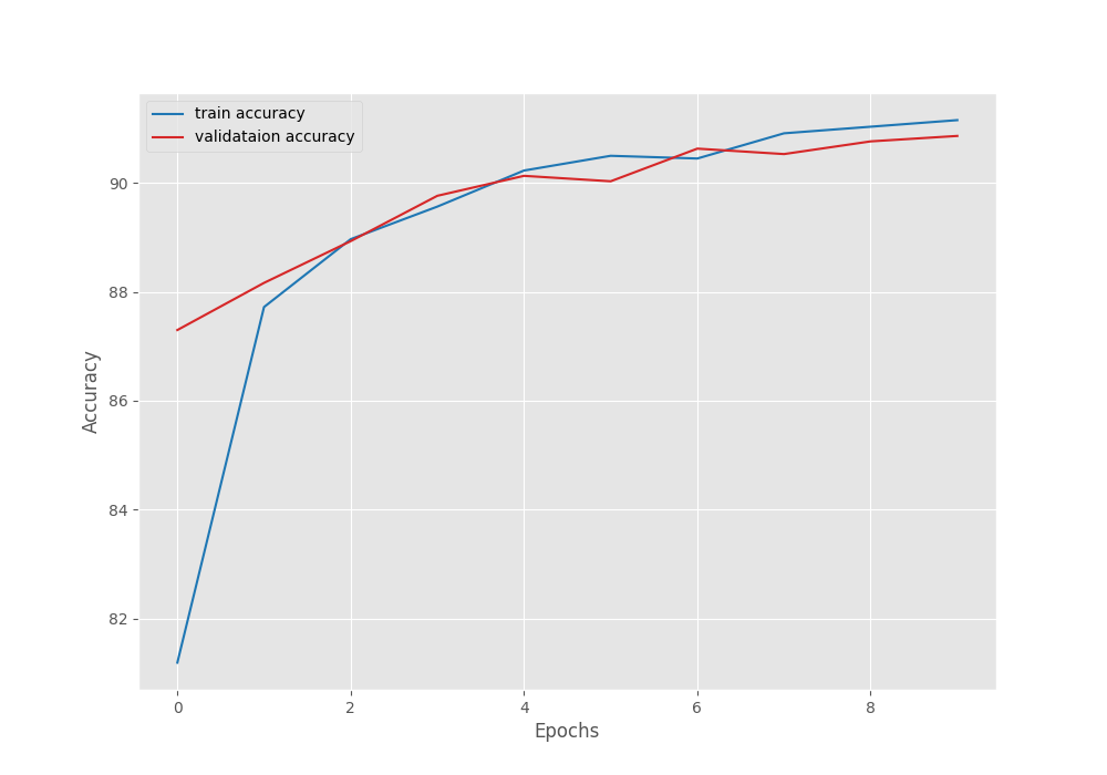
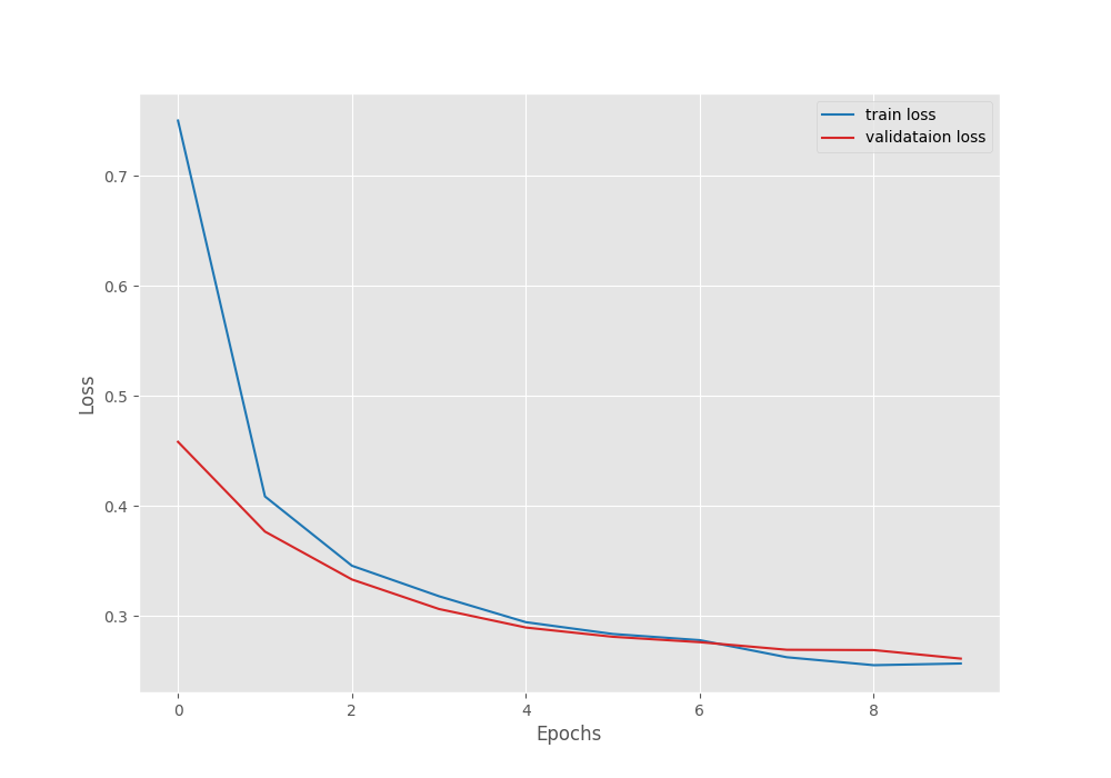
We can see that there is no indication of overfitting. So, most probably, we can train for even longer.

Fine-tuning using IMAGENET1K_V1 Weights

Now, let’s train all the layers using the IMAGENET1K_V1 weights.

python train.py --epochs 10 --weights IMAGENET1K_V1 --batch-size 64 --learning-rate 0.0005 --fine-tune

This time, we pass the --fine-tune flag to train all the intermediate layers.

[INFO]: Number of training images: 14034
[INFO]: Number of validation images: 3000
[INFO]: Classes: ['buildings', 'forest', 'glacier', 'mountain', 'sea', 'street']
Computation device: cuda
Learning rate: 0.0005
Epochs to train for: 10

[INFO]: Loading IMAGENET1K_V1 pre-trained weights
[INFO]: Fine-tuning all layers...
23,520,326 total parameters.
23,520,326 training parameters.
[INFO]: Epoch 1 of 10
Training
100%|██████████████████████████████████████████████████████████████████| 220/220 [00:43<00:00,  5.02it/s]
Validation
100%|████████████████████████████████████████████████████████████████████| 47/47 [00:03<00:00, 14.00it/s]
Training loss: 0.432, training acc: 84.844
Validation loss: 0.378, validation acc: 85.367
--------------------------------------------------
[INFO]: Epoch 2 of 10
Training
100%|██████████████████████████████████████████████████████████████████| 220/220 [00:40<00:00,  5.40it/s]
Validation
100%|████████████████████████████████████████████████████████████████████| 47/47 [00:02<00:00, 16.00it/s]
Training loss: 0.308, training acc: 89.062
Validation loss: 0.317, validation acc: 88.767
--------------------------------------------------
.
.
.
[INFO]: Epoch 10 of 10
Training
100%|██████████████████████████████████████████████████████████████████| 220/220 [00:41<00:00,  5.31it/s]
Validation
100%|████████████████████████████████████████████████████████████████████| 47/47 [00:02<00:00, 16.06it/s]
Training loss: 0.134, training acc: 95.055
Validation loss: 0.267, validation acc: 91.667
--------------------------------------------------
TRAINING COMPLETE

Wow! This time, we have higher validation accuracy compared to both of the previous cases.

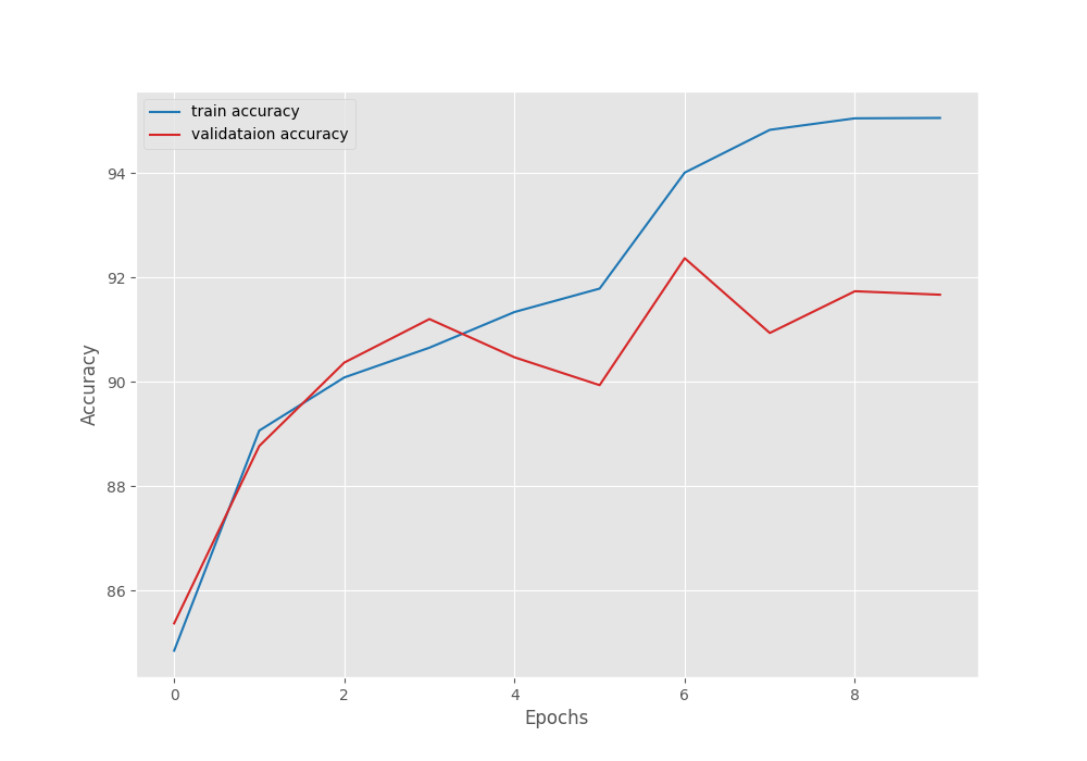
But we can also see much more fluctuation in both, the validation loss and validation accuracy plots. Most probably, we can use a lower learning rate when tuning all layers.

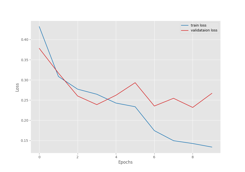
Fine-tuning using IMAGENET1K_V2 Weights

This is the final experiment that we will carry out for comparing the PyTorch IMAGENET1K_V1 and IMAGENET1K_V2 weights. We will use the new ImageNet weights and train all the layers.

python train.py --epochs 10 --weights IMAGENET1K_V2 --batch-size 64 --learning-rate 0.0005 --fine-tune

[INFO]: Number of training images: 14034
[INFO]: Number of validation images: 3000
[INFO]: Classes: ['buildings', 'forest', 'glacier', 'mountain', 'sea', 'street']
Computation device: cuda
Learning rate: 0.0001
Epochs to train for: 10

[INFO]: Loading IMAGENET1K_V2 pre-trained weights
[INFO]: Fine-tuning all layers...
23,520,326 total parameters.
23,520,326 training parameters.
[INFO]: Epoch 1 of 10
Training
100%|██████████████████████████████████████████████████████████████████| 220/220 [00:43<00:00,  5.02it/s]
Validation
100%|████████████████████████████████████████████████████████████████████| 47/47 [00:03<00:00, 14.08it/s]
Training loss: 0.389, training acc: 88.079
Validation loss: 0.194, validation acc: 93.000
--------------------------------------------------
[INFO]: Epoch 2 of 10
Training
100%|██████████████████████████████████████████████████████████████████| 220/220 [00:40<00:00,  5.42it/s]
Validation
100%|████████████████████████████████████████████████████████████████████| 47/47 [00:02<00:00, 15.98it/s]
Training loss: 0.182, training acc: 93.559
Validation loss: 0.167, validation acc: 93.600
--------------------------------------------------
.
.
.
[INFO]: Epoch 10 of 10
Training
100%|██████████████████████████████████████████████████████████████████| 220/220 [00:40<00:00,  5.40it/s]
Validation
100%|████████████████████████████████████████████████████████████████████| 47/47 [00:02<00:00, 16.04it/s]
Training loss: 0.019, training acc: 99.416
Validation loss: 0.211, validation acc: 93.833
Epoch 00010: reducing learning rate of group 0 to 6.2500e-06.
--------------------------------------------------
TRAINING COMPLETE

We have the highest validation accuracy of 93.83% here among all the experiments. Also, the validation loss is the lowest.

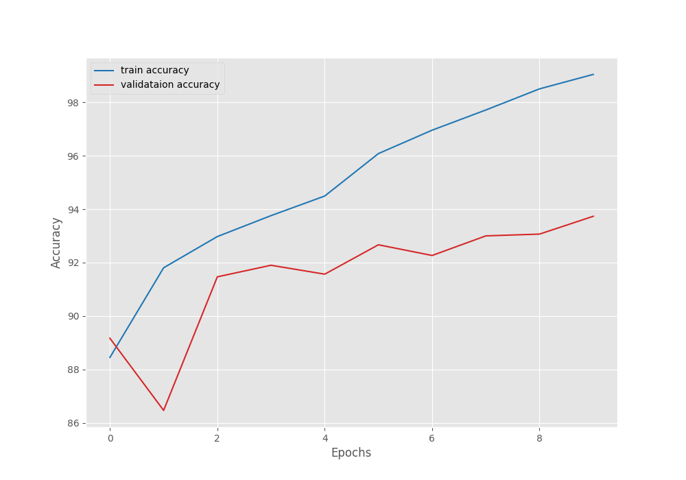
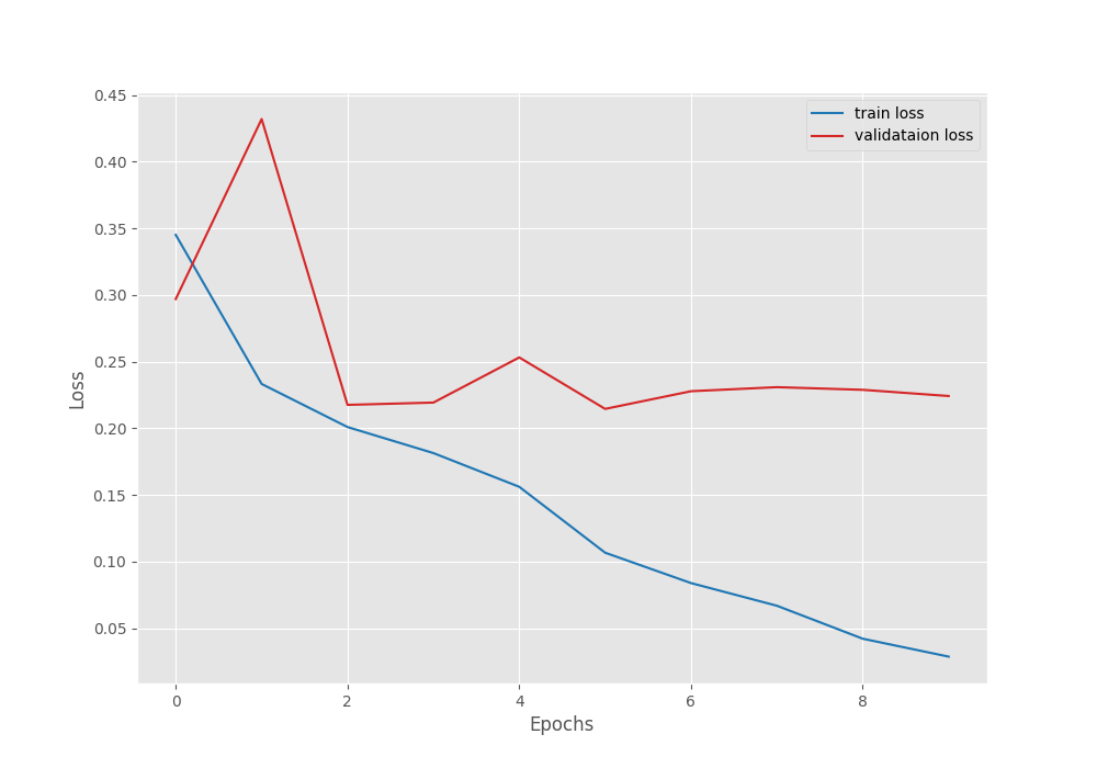
One interesting thing that we can observe here is that the validation plots seem more stable than the IMAGENET1K_V1 weights. Most probably, this is due to the improved pretrained weights.

Takeaways and Further Experiments

The above experiments clearly show that the new ImageNet weights do indeed help in transfer learning and fine-tuning. This means that we can use the same models as before and just train them using the new weights to obtain a better model on a custom dataset. That too without any increased inference cost or trainable parameter!

If you want to do more experiments, you may lower the learning rate while fine-tuning (maybe use 0.0001) and train for longer to see the effects. If you do so, let us know your results in the comment section.

Summary and Conclusion

In this blog post, we carried out experiments for comparison of the PyTorch IMAGENET1K_V1 and IMAGENET1K_V2 weights. From the results, we can conclude that the new ImageNet weights are giving better accuracy in transfer-learning and fine-tuning tasks. I hope that this post was helpful to you.

If you have any doubts, thoughts, or suggestions, please leave them in the comment section. I will surely address them.

You can contact me using the Contact section. You can also find me on LinkedIn, and Twitter.