A Simple Pipeline to Train PyTorch Faster RCNN Object Detection Model

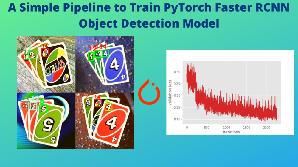
In one of the previous posts, we saw how to train the PyTorch Faster RCNN model on a custom dataset. That was a good starting point of a simple pipeline that we can use to train the PyTorch Faster RCNN model for object detection. So, in this tutorial, we will see how to use the pipeline (and slightly improve upon it) to try to train the PyTorch Faster RCNN model for object detection on any custom dataset.

Note that most of the code will remain similar to what we did in the previous PyTorch Faster RCNN model training post. There are a few changes (small but significant) that we will see in this post. Let’s check out what all we will cover and what are all the changes.

• The code is much simpler now. Almost any dataset that is in Pascal VOC format can be used to train the model.
• The utility code and training code sit separately now making it significantly easier to change in the future.
• You will be getting a zip file with all the scripts in this post. You will also have access to the GitHub repo, which I intend to maintain for considerable time into the future.
• We will check our PyTorch Faster RCNN model training pipeline using the Uno Cards dataset from Roboflow.
• Before going into the training, we will explore the Uno Cards datasetset and try to understand the types of images we have.

As most of the code will remain similar to the previous post, the code explanation will be minimal here. We will focus on the major changes and just go through a high-level explanation of the script. You can think of this post as less of a tutorial and more of a framework/repo explanation. Any suggestion is highly appreciated

Let’s start with knowing more about the dataset.

The Uno Cards Detection Dataset

To train the PyTorch Faster RCNN model for object detection, we will use the Uno Cards dataset from Roboflow here.

If you visit the website, you will find that there are two different versions of the dataset. They are:

• raw: These contain the the original 8992 images.
• v1: This is an augmented version of the dataset containing 21582 images.

The raw Dataset Version

To keep the training time short, we will use the original raw version of the dataset.

To be fair, the original version is not that small as well. It still contains almost 9000 images and around 30000 annotations. We have a good amount of data here.

The dataset consists of 15 classes in total.

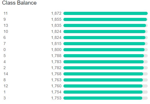
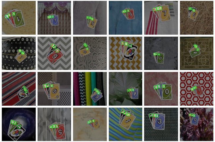
The above figure shows the distribution of images across different classes. Still, it does not give us a good idea of which labels correspond to which images/objects in the dataset. These are just numbers. Let’s try to demystify that first.

Okay! This gives us a much better idea about the images and the corresponding classes.

• Numbers 0 to 9 on the card have the same labels, that is, 0 to 9. That’s 10 labels there.
• Label 10 corresponds to +4 on card.
• Label 11 is +2 on the card.
• The double arrow on the card has a mapping to label 12.
• The phi (\(\phi\)) corresponds to label 13.
• And finally, the colored circle (or wildcard symbol) is label 14.

The above points obviously do not contain the exact terms of Uno cards. But it is helpful enough for us so that we can deal with the deep learning stuff and know whether our model is correctly predicting everything or not. If you want to know about Uno cards, consider visiting this link.

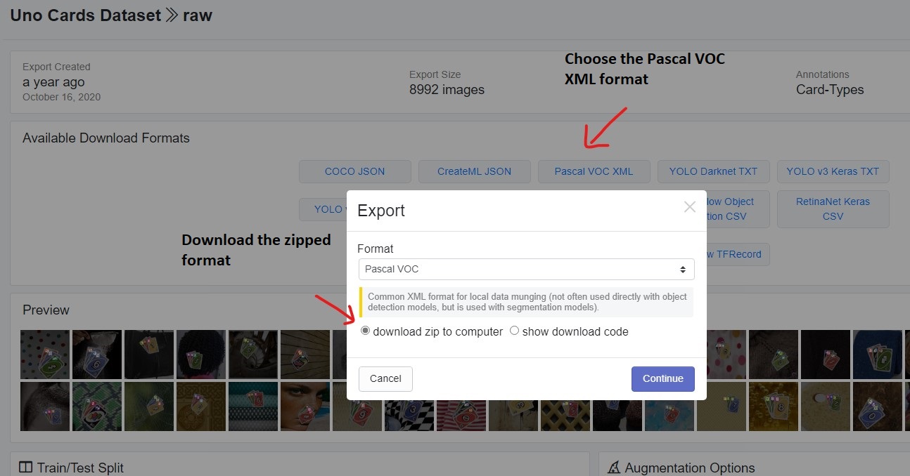
Before moving further, it is important that you download the dataset from this link. Download the Pascal VOC XML format as shown in the image below.

The Directory Structure

The following block shows the directory structure that we will use for this project.

│   config.py
│   custom_utils.py
│   datasets.py
│   inference.py
│   inference_video.py
│   model.py
│   train.py
├───data
│   ├───Uno Cards.v2-raw.voc
│   │   ├───test
│   │   ├───train
│   │   └───valid
│   └───uno_custom_test_data
├───inference_outputs
│   ├───images
│   └───videos
├───outputs
│   ├───best_model.pth
│   ├───last_model.pth
│   ├───train_loss.png
│   ├───valid_loss.png

• We have 7 Python files. We will not go into the details of the content of these yet. It will be much more beneficial to discuss these when we enter the coding section.
• The data directory contains the Uno Cards datasets. After downloading the dataset, be sure to extract it and have it in the same structure as above. The train, valid, and test subdirectories contain the JPG images and the corresponding XML files for the annotations.
• The inference_outputs directory will contain all the outputs that we will be genered by running the inference.py and inference_video.py script.
• Then we have the outputs directory. This will hold the trained models and loss graphs when we carry out the training.

If you have downloaded the zip file for this post, then you already have almost everything in place. You just need to extract the dataset in the correct structure inside the data directory.

Downloading the code files will also give you access to the trained models. You need not train the models again as that can be a time-consuming and resource-intensive process. If you wish, you may train for a few iterations just to check how the training is going and move on to the next phase in the post.

The PyTorch Version

We will use PyTorch 1.10 for coding out the Faster RCNN training pipeline. It is the latest version of PyTorch at the time of writing this post.

You may choose to use whatever new version of PyTorch that is available when you are reading this. Hopefully, everything will run fine.

Other Library Dependencies

The code uses other common computer vision libraries like OpenCV and Albumentations. You may install them as you code along if you don’t already have them. While installing the Albumentations library, be sure to install the latest version as many new features get added frequently into it.

We will use the Albumentations library for image augmentation for object detection. If you want to learn more about the topic, please refer to these two tutorials:

• Bounding Box Augmentation for Object Detection using Albumentations
• Applying Different Augmentations to Bounding Boxes in Object Detection using Albumentations

Code to Train the PyTorch Faster RCNN Model

From here onward, we will start with the coding part of the post. As discussed earlier, we will not get into the very details of the code. Rather, we will try to understand what each Python file does on a high level. Although some of the code has changed along with a few file names, you can refer to this post for a detailed explanation of the code.

We have seven Python files with us. Let’s tackle each of them in the following order:

• config.py
• custom_utils.py
• datasets.py
• model.py
• train.py
• inference.py
• inference_video.py

Let’s start with the configuration file.

Setting Up the Training Configuration

We will write all the training configurations in the config.py file.

The following block contains the entire code that we need for the file.

import torch

BATCH_SIZE = 8 # increase / decrease according to GPU memeory
RESIZE_TO = 416 # resize the image for training and transforms
NUM_EPOCHS = 10 # number of epochs to train for
NUM_WORKERS = 4

DEVICE = torch.device('cuda') if torch.cuda.is_available() else torch.device('cpu')

# training images and XML files directory
TRAIN_DIR = 'data/Uno Cards.v2-raw.voc/train'
# validation images and XML files directory
VALID_DIR = 'data/Uno Cards.v2-raw.voc/valid'

# classes: 0 index is reserved for background
CLASSES = [
    '__background__', '11', '9', '13', '10', '6', '7', '0', '5', '4', '2', '14', 
    '8', '12', '1', '3'
]

NUM_CLASSES = len(CLASSES)

# whether to visualize images after crearing the data loaders
VISUALIZE_TRANSFORMED_IMAGES = True

# location to save model and plots
OUT_DIR = 'outputs'

The training configuration file contains the following information:

• The batch size to use for training. If you carry out training on your own system, then you may increase or decrease the size according to your available GPU memory.
• The dimensions that we want the images to resize to, that is RESIZE_TO.
• Number of epochs to train for. The models included in the zip file for download are trained for 10 epochs as well.
• Number of workers or sub-processes to use for data loading. This helps a lot when we have a large dataset or reading images form disk, or even doing a lot of image augmentations as well.
• The computation device to use for training. For training, you will need a GPU. A CPU is just too slow for Faster RCNN training and object detection training in general as well.
• The TRAIN_DIR is a string containing the path to the training images and XML files. Similar for VALID_DIR for the validation images and XML files.
• Then we have the classes and the number of classes. Note that we have a __background__ class at the beginning. This is required while fine-tuning PyTorch object detection models. The class at index 0 is always the __background__ class.
• VISUALIZE_TRANSFORMED_IMAGES controls whether we want to visualize the data loader images or not just before training.
• OUT_DIR contains the path to the directory to store the trained models and the loss graphs.

That’s all we have for the training configuration file.

Helper Functions and Utility Classes

Next, we need to define a few helper functions and utility classes. These are small yet very convenient pieces of code that will help us a lot while training the model. There are a total of two classes and 6 functions.

This code will go into the custom_utils.py file.

Let’s take a look at the code. First, the utility classes.

import albumentations as A
import cv2
import numpy as np
import torch
import matplotlib.pyplot as plt

from albumentations.pytorch import ToTensorV2
from config import DEVICE, CLASSES

plt.style.use('ggplot')

# this class keeps track of the training and validation loss values...
# ... and helps to get the average for each epoch as well
class Averager:
    def __init__(self):
        self.current_total = 0.0
        self.iterations = 0.0
        
    def send(self, value):
        self.current_total += value
        self.iterations += 1
    
    @property
    def value(self):
        if self.iterations == 0:
            return 0
        else:
            return 1.0 * self.current_total / self.iterations
    
    def reset(self):
        self.current_total = 0.0
        self.iterations = 0.0

class SaveBestModel:
    """
    Class to save the best model while training. If the current epoch's 
    validation loss is less than the previous least less, then save the
    model state.
    """
    def __init__(
        self, best_valid_loss=float('inf')
    ):
        self.best_valid_loss = best_valid_loss
        
    def __call__(
        self, current_valid_loss, 
        epoch, model, optimizer
    ):
        if current_valid_loss < self.best_valid_loss:
            self.best_valid_loss = current_valid_loss
            print(f"\nBest validation loss: {self.best_valid_loss}")
            print(f"\nSaving best model for epoch: {epoch+1}\n")
            torch.save({
                'epoch': epoch+1,
                'model_state_dict': model.state_dict(),
                'optimizer_state_dict': optimizer.state_dict(),
                }, 'outputs/best_model.pth')

• The Averager class is for keeping track of the training and validation loss values. We can also retrieve the average loss after each epoch with help of instances of this class. You may spend some time to properly understand it if you are new to such an Averager class.
• The SaveBestModel class is a very simple function to save the best model after each epoch. We call the instance of this class while passing the current epoch’s validation loss. If that is the best loss, then a new best model is saved to the disk.

Next, the helper functions.

def collate_fn(batch):
    """
    To handle the data loading as different images may have different number 
    of objects and to handle varying size tensors as well.
    """
    return tuple(zip(*batch))

# define the training tranforms
def get_train_transform():
    return A.Compose([
        A.Flip(0.5),
        A.RandomRotate90(0.5),
        A.MotionBlur(p=0.2),
        A.MedianBlur(blur_limit=3, p=0.1),
        A.Blur(blur_limit=3, p=0.1),
        ToTensorV2(p=1.0),
    ], bbox_params={
        'format': 'pascal_voc',
        'label_fields': ['labels']
    })

# define the validation transforms
def get_valid_transform():
    return A.Compose([
        ToTensorV2(p=1.0),
    ], bbox_params={
        'format': 'pascal_voc', 
        'label_fields': ['labels']
    })


def show_tranformed_image(train_loader):
    """
    This function shows the transformed images from the `train_loader`.
    Helps to check whether the tranformed images along with the corresponding
    labels are correct or not.
    Only runs if `VISUALIZE_TRANSFORMED_IMAGES = True` in config.py.
    """
    if len(train_loader) > 0:
        for i in range(1):
            images, targets = next(iter(train_loader))
            images = list(image.to(DEVICE) for image in images)
            targets = [{k: v.to(DEVICE) for k, v in t.items()} for t in targets]
            boxes = targets[i]['boxes'].cpu().numpy().astype(np.int32)
            labels = targets[i]['labels'].cpu().numpy().astype(np.int32)
            sample = images[i].permute(1, 2, 0).cpu().numpy()
            for box_num, box in enumerate(boxes):
                cv2.rectangle(sample,
                            (box[0], box[1]),
                            (box[2], box[3]),
                            (0, 0, 255), 2)
                cv2.putText(sample, CLASSES[labels[box_num]], 
                            (box[0], box[1]-10), cv2.FONT_HERSHEY_SIMPLEX, 
                            1.0, (0, 0, 255), 2)
            cv2.imshow('Transformed image', sample)
            cv2.waitKey(0)
            cv2.destroyAllWindows()

def save_model(epoch, model, optimizer):
    """
    Function to save the trained model till current epoch, or whenver called
    """
    torch.save({
                'epoch': epoch+1,
                'model_state_dict': model.state_dict(),
                'optimizer_state_dict': optimizer.state_dict(),
                }, 'outputs/last_model.pth')

def save_loss_plot(OUT_DIR, train_loss, val_loss):
    figure_1, train_ax = plt.subplots()
    figure_2, valid_ax = plt.subplots()
    train_ax.plot(train_loss, color='tab:blue')
    train_ax.set_xlabel('iterations')
    train_ax.set_ylabel('train loss')
    valid_ax.plot(val_loss, color='tab:red')
    valid_ax.set_xlabel('iterations')
    valid_ax.set_ylabel('validation loss')
    figure_1.savefig(f"{OUT_DIR}/train_loss.png")
    figure_2.savefig(f"{OUT_DIR}/valid_loss.png")
    print('SAVING PLOTS COMPLETE...')

    plt.close('all')

• The collate_fn() will help us take care of tensors of varying sizes while creating the training and validation data loaders.
• Then we have the get_train_transform() and get_valid_transform() functions defining the data augmentations for the images. Note that the dataset format is pascal_voc, which is pretty important to mention correctly.
• The show_tranformed_image() is for showing the image from the training data loader just before the training begins. This will helps us check that the augmented images and the bounding boxes are indeed correct.
• Then we have function to save the model after each epoch and after training ends.
• And another function to save the training and validation loss graphs. This will be called after each epoch.

This completes the code for the custom_utils.py file as well.

Prepare the Dataset

Preparing the dataset correctly is really important for object detection training. Any small mistake while loading the bounding box coordinates can throw of training entirely.

We will not go into a detailed explanation of the dataset preparation process here. In the Custom Object Detection using PyTorch Faster RCNN we went over the code in detail. Although the dataset is different here, there is almost no difference in the custom dataset preparation class. Please go over mentioned post to get a detailed view of the code here.

This code will be in the datasets.py file.

import torch
import cv2
import numpy as np
import os
import glob as glob

from xml.etree import ElementTree as et
from config import (
    CLASSES, RESIZE_TO, TRAIN_DIR, VALID_DIR, BATCH_SIZE
)
from torch.utils.data import Dataset, DataLoader
from custom_utils import collate_fn, get_train_transform, get_valid_transform

# the dataset class
class CustomDataset(Dataset):
    def __init__(self, dir_path, width, height, classes, transforms=None):
        self.transforms = transforms
        self.dir_path = dir_path
        self.height = height
        self.width = width
        self.classes = classes
        
        # get all the image paths in sorted order
        self.image_paths = glob.glob(f"{self.dir_path}/*.jpg")
        self.all_images = [image_path.split(os.path.sep)[-1] for image_path in self.image_paths]
        self.all_images = sorted(self.all_images)

    def __getitem__(self, idx):
        # capture the image name and the full image path
        image_name = self.all_images[idx]
        image_path = os.path.join(self.dir_path, image_name)

        # read the image
        image = cv2.imread(image_path)
        # convert BGR to RGB color format
        image = cv2.cvtColor(image, cv2.COLOR_BGR2RGB).astype(np.float32)
        image_resized = cv2.resize(image, (self.width, self.height))
        image_resized /= 255.0
        
        # capture the corresponding XML file for getting the annotations
        annot_filename = image_name[:-4] + '.xml'
        annot_file_path = os.path.join(self.dir_path, annot_filename)
        
        boxes = []
        labels = []
        tree = et.parse(annot_file_path)
        root = tree.getroot()
        
        # get the height and width of the image
        image_width = image.shape[1]
        image_height = image.shape[0]
        
        # box coordinates for xml files are extracted and corrected for image size given
        for member in root.findall('object'):
            # map the current object name to `classes` list to get...
            # ... the label index and append to `labels` list
            labels.append(self.classes.index(member.find('name').text))
            
            # xmin = left corner x-coordinates
            xmin = int(member.find('bndbox').find('xmin').text)
            # xmax = right corner x-coordinates
            xmax = int(member.find('bndbox').find('xmax').text)
            # ymin = left corner y-coordinates
            ymin = int(member.find('bndbox').find('ymin').text)
            # ymax = right corner y-coordinates
            ymax = int(member.find('bndbox').find('ymax').text)
            
            # resize the bounding boxes according to the...
            # ... desired `width`, `height`
            xmin_final = (xmin/image_width)*self.width
            xmax_final = (xmax/image_width)*self.width
            ymin_final = (ymin/image_height)*self.height
            yamx_final = (ymax/image_height)*self.height
            
            boxes.append([xmin_final, ymin_final, xmax_final, yamx_final])
        
        # bounding box to tensor
        boxes = torch.as_tensor(boxes, dtype=torch.float32)
        # area of the bounding boxes
        area = (boxes[:, 3] - boxes[:, 1]) * (boxes[:, 2] - boxes[:, 0])
        # no crowd instances
        iscrowd = torch.zeros((boxes.shape[0],), dtype=torch.int64)
        # labels to tensor
        labels = torch.as_tensor(labels, dtype=torch.int64)

        # prepare the final `target` dictionary
        target = {}
        target["boxes"] = boxes
        target["labels"] = labels
        target["area"] = area
        target["iscrowd"] = iscrowd
        image_id = torch.tensor([idx])
        target["image_id"] = image_id

        # apply the image transforms
        if self.transforms:
            sample = self.transforms(image = image_resized,
                                     bboxes = target['boxes'],
                                     labels = labels)
            image_resized = sample['image']
            target['boxes'] = torch.Tensor(sample['bboxes'])
            
        return image_resized, target

    def __len__(self):
        return len(self.all_images)

# prepare the final datasets and data loaders
def create_train_dataset():
    train_dataset = CustomDataset(TRAIN_DIR, RESIZE_TO, RESIZE_TO, CLASSES, get_train_transform())
    return train_dataset
def create_valid_dataset():
    valid_dataset = CustomDataset(VALID_DIR, RESIZE_TO, RESIZE_TO, CLASSES, get_valid_transform())
    return valid_dataset

def create_train_loader(train_dataset, num_workers=0):
    train_loader = DataLoader(
        train_dataset,
        batch_size=BATCH_SIZE,
        shuffle=True,
        num_workers=num_workers,
        collate_fn=collate_fn
    )
    return train_loader
def create_valid_loader(valid_dataset, num_workers=0):
    valid_loader = DataLoader(
        valid_dataset,
        batch_size=BATCH_SIZE,
        shuffle=False,
        num_workers=num_workers,
        collate_fn=collate_fn
    )
    return valid_loader


# execute datasets.py using Python command from Terminal...
# ... to visualize sample images
# USAGE: python datasets.py
if __name__ == '__main__':
    # sanity check of the Dataset pipeline with sample visualization
    dataset = CustomDataset(
        TRAIN_DIR, RESIZE_TO, RESIZE_TO, CLASSES
    )
    print(f"Number of training images: {len(dataset)}")
    
    # function to visualize a single sample
    def visualize_sample(image, target):
        for box_num in range(len(target['boxes'])):
            box = target['boxes'][box_num]
            label = CLASSES[target['labels'][box_num]]
            cv2.rectangle(
                image, 
                (int(box[0]), int(box[1])), (int(box[2]), int(box[3])),
                (0, 255, 0), 2
            )
            cv2.putText(
                image, label, (int(box[0]), int(box[1]-5)), 
                cv2.FONT_HERSHEY_SIMPLEX, 0.7, (0, 0, 255), 2
            )
        cv2.imshow('Image', image)
        cv2.waitKey(0)
        
    NUM_SAMPLES_TO_VISUALIZE = 5
    for i in range(NUM_SAMPLES_TO_VISUALIZE):
        image, target = dataset[i]
        visualize_sample(image, target)

Yes, this is a long piece of code. But once you understand it, you can use it for any object detection dataset preparation that is in the Pascal VOC format.

The Faster RCNN Model with ResNet50 Backbone

The model preparation part is quite easy and straightforward. PyTorch already provides a pre-trained Faster RCNN ResNet50 FPN model. So, we just need to:

• Load that model.
• Get the number of input features.
• And add a new head with the correct number of classes according to our dataset.

Writing the model preparation code in model.py file.

import torchvision

from torchvision.models.detection.faster_rcnn import FastRCNNPredictor

def create_model(num_classes):
    
    # load Faster RCNN pre-trained model
    model = torchvision.models.detection.fasterrcnn_resnet50_fpn(pretrained=True)
    
    # get the number of input features 
    in_features = model.roi_heads.box_predictor.cls_score.in_features
    # define a new head for the detector with required number of classes
    model.roi_heads.box_predictor = FastRCNNPredictor(in_features, num_classes) 

    return model

The above block contains all the code that we need to prepare the Faster RCNN model with the ResNet50 FPN backbone. It’s perhaps one of the easiest parts of the entire process.

The Training Code

If you go over the Faster RCNN training post for Microcontroller detection, then you would realize that we had the runnable training code in engine.py file. For convenience, let’s rename that to train.py.

The code will remain almost the same. Just a bit more modular and customizable. A few issues with Windows multi-processing (num_workers>0) has been solved. So, training on both Ubuntu and Windows OS should relatively take the same time.

The training code will go into the train.py file.

The first code block contains the import statements that we need.

from config import (
    DEVICE, NUM_CLASSES, NUM_EPOCHS, OUT_DIR,
    VISUALIZE_TRANSFORMED_IMAGES, NUM_WORKERS,
)
from model import create_model
from custom_utils import Averager, SaveBestModel, save_model, save_loss_plot
from tqdm.auto import tqdm
from datasets import (
    create_train_dataset, create_valid_dataset, 
    create_train_loader, create_valid_loader
)

import torch
import matplotlib.pyplot as plt
import time

plt.style.use('ggplot')

We have imported all the required modules that we have written on our own. Along with that, we also import torch and matplotlib for plotting.

Next, the training function.

# function for running training iterations
def train(train_data_loader, model):
    print('Training')
    global train_itr
    global train_loss_list
    
     # initialize tqdm progress bar
    prog_bar = tqdm(train_data_loader, total=len(train_data_loader))
    
    for i, data in enumerate(prog_bar):
        optimizer.zero_grad()
        images, targets = data
        
        images = list(image.to(DEVICE) for image in images)
        targets = [{k: v.to(DEVICE) for k, v in t.items()} for t in targets]

        loss_dict = model(images, targets)

        losses = sum(loss for loss in loss_dict.values())
        loss_value = losses.item()
        train_loss_list.append(loss_value)

        train_loss_hist.send(loss_value)

        losses.backward()
        optimizer.step()

        train_itr += 1
    
        # update the loss value beside the progress bar for each iteration
        prog_bar.set_description(desc=f"Loss: {loss_value:.4f}")
    return train_loss_list

The training function always returns a list containing the training loss values for all the completed iterations.

Now, the validation function.

# function for running validation iterations
def validate(valid_data_loader, model):
    print('Validating')
    global val_itr
    global val_loss_list
    
    # initialize tqdm progress bar
    prog_bar = tqdm(valid_data_loader, total=len(valid_data_loader))
    
    for i, data in enumerate(prog_bar):
        images, targets = data
        
        images = list(image.to(DEVICE) for image in images)
        targets = [{k: v.to(DEVICE) for k, v in t.items()} for t in targets]
        
        with torch.no_grad():
            loss_dict = model(images, targets)

        losses = sum(loss for loss in loss_dict.values())
        loss_value = losses.item()
        val_loss_list.append(loss_value)

        val_loss_hist.send(loss_value)

        val_itr += 1

        # update the loss value beside the progress bar for each iteration
        prog_bar.set_description(desc=f"Loss: {loss_value:.4f}")
    return val_loss_list

The validation function returns a similar list containing the loss values for all the completed iterations.

The only remaining part of the script is the main training block. Let’s take a look

if __name__ == '__main__':
    train_dataset = create_train_dataset()
    valid_dataset = create_valid_dataset()
    train_loader = create_train_loader(train_dataset, NUM_WORKERS)
    valid_loader = create_valid_loader(valid_dataset, NUM_WORKERS)
    print(f"Number of training samples: {len(train_dataset)}")
    print(f"Number of validation samples: {len(valid_dataset)}\n")

    # initialize the model and move to the computation device
    model = create_model(num_classes=NUM_CLASSES)
    model = model.to(DEVICE)
    # get the model parameters
    params = [p for p in model.parameters() if p.requires_grad]
    # define the optimizer
    optimizer = torch.optim.SGD(params, lr=0.001, momentum=0.9, weight_decay=0.0005)

    # initialize the Averager class
    train_loss_hist = Averager()
    val_loss_hist = Averager()
    train_itr = 1
    val_itr = 1
    # train and validation loss lists to store loss values of all...
    # ... iterations till ena and plot graphs for all iterations
    train_loss_list = []
    val_loss_list = []

    # name to save the trained model with
    MODEL_NAME = 'model'

    # whether to show transformed images from data loader or not
    if VISUALIZE_TRANSFORMED_IMAGES:
        from custom_utils import show_tranformed_image
        show_tranformed_image(train_loader)

    # initialize SaveBestModel class
    save_best_model = SaveBestModel()

    # start the training epochs
    for epoch in range(NUM_EPOCHS):
        print(f"\nEPOCH {epoch+1} of {NUM_EPOCHS}")

        # reset the training and validation loss histories for the current epoch
        train_loss_hist.reset()
        val_loss_hist.reset()

        # start timer and carry out training and validation
        start = time.time()
        train_loss = train(train_loader, model)
        val_loss = validate(valid_loader, model)
        print(f"Epoch #{epoch+1} train loss: {train_loss_hist.value:.3f}")   
        print(f"Epoch #{epoch+1} validation loss: {val_loss_hist.value:.3f}")   
        end = time.time()
        print(f"Took {((end - start) / 60):.3f} minutes for epoch {epoch}")

        # save the best model till now if we have the least loss in the...
        # ... current epoch
        save_best_model(
            val_loss_hist.value, epoch, model, optimizer
        )
        # save the current epoch model
        save_model(epoch, model, optimizer)

        # save loss plot
        save_loss_plot(OUT_DIR, train_loss, val_loss)
        
        # sleep for 5 seconds after each epoch
        time.sleep(5)

This is almost similar to the main training block here. The only difference is that we are now saving the best model, and the last epoch’s model separately instead of saving the model after specific intervals. And the model saving and plotting functions are now handled by the cusom_utils module.

With this, we complete our training code as well. In the next section, we will execute this script and take a look at how well the model is learning.

Execute train.py to Train the Model

Open your terminal/command prompt within the project directory where the train.py script is present.

Note: You need not train the model if you do not have access to a GPU. You already have access to the trained model when you download the zip file. You may read through this section, and move on to the inference part of the post.

Execute the following command to train the model for 10 epochs.

python train.py

The following block shows the output in a truncated format.

Number of training samples: 6295
Number of validation samples: 1798

Downloading: "https://download.pytorch.org/models/fasterrcnn_resnet50_fpn_coco-258fb6c6.pth" to /root/.cache/torch/hub/checkpoints/fasterrcnn_resnet50_fpn_coco-258fb6c6.pth
100%
160M/160M [00:07<00:00, 23.3MB/s]
EPOCH 1 of 10
Training
Loss: 0.3155: 100%
787/787 [11:27<00:00, 1.18it/s]
Validating
Loss: 0.2686: 100%
225/225 [01:42<00:00, 2.44it/s]
Epoch #1 train loss: 0.554
Epoch #1 validation loss: 0.272
Took 13.165 minutes for epoch 0

Best validation loss: 0.27201075739330716

Saving best model for epoch: 1

SAVING PLOTS COMPLETE...
...
...
...
EPOCH 10 of 10
Training
Loss: 0.1379: 100%
787/787 [11:23<00:00, 1.18it/s]
Validating
Loss: 0.1191: 100%
225/225 [01:42<00:00, 2.37it/s]
Epoch #10 train loss: 0.137
Epoch #10 validation loss: 0.123
Took 13.097 minutes for epoch 9

Best validation loss: 0.12344141857491599

Saving best model for epoch: 10

SAVING PLOTS COMPLETE...

By the end of 10 epochs, we have the best validation loss of 0.1234. If you train the model on your own, your results might vary a bit. But they should be pretty close.

Now, let’s take a look at the training and validation loss graphs.

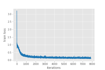
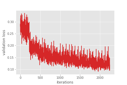
These look pretty good. The validation loss is clearly decreasing till the end of training. For the training loss, although, it looks to plateau around 5000 iterations, it is actually decreasing.

As our training is complete now, we will start with the inference part in the next section.

Carrying Out Inference on Images

If you remember, we already have a test folder for the Uno Cards dataset that we did not use for training. It contains the images and XML files. We will use these images to carry out inference.

We will not need the XML files, as the images are just enough to get the predictions by doing a forward pass through the trained model.

The inference script is almost the same as we wrote in the Microcontroller detection post. Only a few minor changes here.

The code for carrying out inference on images will go into the inference.py file.

Starting with the imports and creating a NumPy array to create different colors for different classes.

import numpy as np
import cv2
import torch
import glob as glob
import os
import time

from model import create_model

from config import (
    NUM_CLASSES, DEVICE, CLASSES
)

# this will help us create a different color for each class
COLORS = np.random.uniform(0, 255, size=(len(CLASSES), 3))

COLORS is a NumPy array that will generate a different color for each of the classes. When annotating the images with bounding boxes, this will help us differentiate between different classes easily.

Now, loading the model, grabbing all the test image paths, and defining the confidence threshold.

# load the best model and trained weights
model = create_model(num_classes=NUM_CLASSES)
checkpoint = torch.load('outputs/best_model.pth', map_location=DEVICE)
model.load_state_dict(checkpoint['model_state_dict'])
model.to(DEVICE).eval()

# directory where all the images are present
DIR_TEST = 'data/Uno Cards.v2-raw.voc/test'
test_images = glob.glob(f"{DIR_TEST}/*.jpg")
print(f"Test instances: {len(test_images)}")

# define the detection threshold...
# ... any detection having score below this will be discarded
detection_threshold = 0.8

# to count the total number of images iterated through
frame_count = 0
# to keep adding the FPS for each image
total_fps = 0 

In the above code block, we have two other variables as well. frame_count will keep track of all the images we iterate through so that we can calculate a final FPS for all the images. And we will keep adding the FPS for each image to total_fps.

Next, iterating through the image paths, and carry out the inference.

for i in range(len(test_images)):
    # get the image file name for saving output later on
    image_name = test_images[i].split(os.path.sep)[-1].split('.')[0]
    image = cv2.imread(test_images[i])
    orig_image = image.copy()
    # BGR to RGB
    image = cv2.cvtColor(orig_image, cv2.COLOR_BGR2RGB).astype(np.float32)
    # make the pixel range between 0 and 1
    image /= 255.0
    # bring color channels to front
    image = np.transpose(image, (2, 0, 1)).astype(np.float32)
    # convert to tensor
    image = torch.tensor(image, dtype=torch.float).cuda()
    # add batch dimension
    image = torch.unsqueeze(image, 0)
    start_time = time.time()
    with torch.no_grad():
        outputs = model(image.to(DEVICE))
    end_time = time.time()

    # get the current fps
    fps = 1 / (end_time - start_time)
    # add `fps` to `total_fps`
    total_fps += fps
    # increment frame count
    frame_count += 1
    # load all detection to CPU for further operations
    outputs = [{k: v.to('cpu') for k, v in t.items()} for t in outputs]
    # carry further only if there are detected boxes
    if len(outputs[0]['boxes']) != 0:
        boxes = outputs[0]['boxes'].data.numpy()
        scores = outputs[0]['scores'].data.numpy()
        # filter out boxes according to `detection_threshold`
        boxes = boxes[scores >= detection_threshold].astype(np.int32)
        draw_boxes = boxes.copy()
        # get all the predicited class names
        pred_classes = [CLASSES[i] for i in outputs[0]['labels'].cpu().numpy()]
        
        # draw the bounding boxes and write the class name on top of it
        for j, box in enumerate(draw_boxes):
            class_name = pred_classes[j]
            color = COLORS[CLASSES.index(class_name)]
            cv2.rectangle(orig_image,
                        (int(box[0]), int(box[1])),
                        (int(box[2]), int(box[3])),
                        color, 2)
            cv2.putText(orig_image, class_name, 
                        (int(box[0]), int(box[1]-5)),
                        cv2.FONT_HERSHEY_SIMPLEX, 0.7, color, 
                        2, lineType=cv2.LINE_AA)

        cv2.imshow('Prediction', orig_image)
        cv2.waitKey(1)
        cv2.imwrite(f"inference_outputs/images/{image_name}.jpg", orig_image)
    print(f"Image {i+1} done...")
    print('-'*50)

print('TEST PREDICTIONS COMPLETE')
cv2.destroyAllWindows()
# calculate and print the average FPS
avg_fps = total_fps / frame_count
print(f"Average FPS: {avg_fps:.3f}")

We do the forward pass on lines 51 and 52. From lines 74 to 84, we annotate the images with the bounding boxes and the predicted class names.

We show the image on the screen for just 1 millisecond. We save images to the disk, which we take a look at later on.

Executing inference.py

Execute the following command to run the inference script on the test images.

python inference.py

You should see output similar to the following on your terminal window.

Image 1 done...
--------------------------------------------------
Image 2 done...
--------------------------------------------------
...
Image 898 done...
--------------------------------------------------
Image 899 done...
--------------------------------------------------
TEST PREDICTIONS COMPLETE
Average FPS: 14.392

So, we are getting an average FPS of around 14 on all the 899 images. Your FPS might vary depending on the hardware that you have.

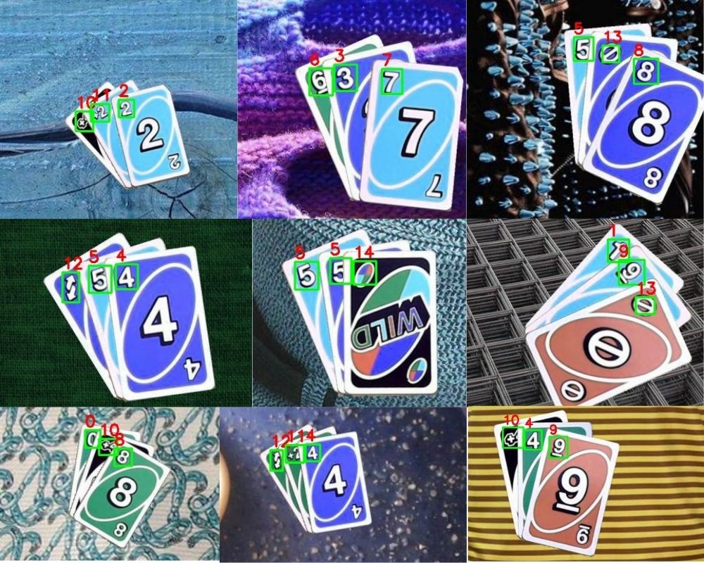
The following image shows a few of the predictions that are saved to disk.

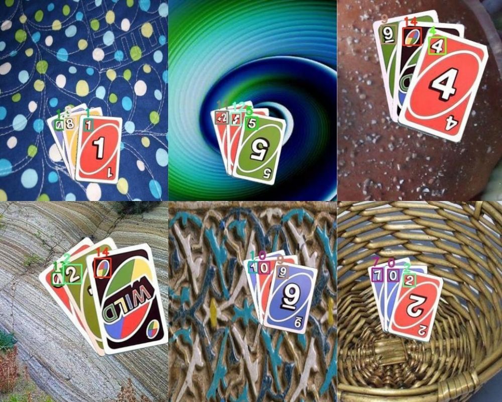
From the above figure, it is pretty clear that all the predictions are correct. In fact, in some of the cases, where the \(\phi\) is almost hidden, then also the model is able to correctly predict the class as 13. That’s pretty good.

Running inference on all the 899 images might take some time. But everything is saved to disk. So, you can analyze the results later.

Carrying Out Inference on Video

Generally, the Faster RCNN ResNet50 model is not meant for real-time video predictions. But why not give it a try and check out how well it predicts when the cards are moving.

One thing to note here is that depending on the hardware (GPU mostly), your FPS will vary a lot. The results in this post are from running the video predictions (and image predictions as well) on an RTX 3080 GPU. So, if you get really low FPS, you can consider skipping this part from a practical perspective and just read through the section.

The code here will go into the inference_video.py file.

The code will mostly be similar to the image inference section. Instead of iterating through images, we will:

• Capture the video using OpenCV.
• Keep on checking if frames are still present to iterate through.
• If a frame is present, apply the same preprocessing as we did for images and forward pass through the model.
• Annotate the bounding boxes, labels, and FPS on the current frame and show the frame on screen.

The following block holds the code for the entire script.

import numpy as np
import cv2
import torch
import os
import time
import argparse
import pathlib

from model import create_model
from config import (
    NUM_CLASSES, DEVICE, CLASSES
)

# construct the argument parser
parser = argparse.ArgumentParser()
parser.add_argument(
    '-i', '--input', help='path to input video',
    default='data/uno_custom_test_data/video_1.mp4'
)
args = vars(parser.parse_args())

# this will help us create a different color for each class
COLORS = np.random.uniform(0, 255, size=(len(CLASSES), 3))

# load the best model and trained weights
model = create_model(num_classes=NUM_CLASSES)
checkpoint = torch.load('outputs/best_model.pth', map_location=DEVICE)
model.load_state_dict(checkpoint['model_state_dict'])
model.to(DEVICE).eval()

# define the detection threshold...
# ... any detection having score below this will be discarded
detection_threshold = 0.8
RESIZE_TO = (512, 512)

cap = cv2.VideoCapture(args['input'])

if (cap.isOpened() == False):
    print('Error while trying to read video. Please check path again')

# get the frame width and height
frame_width = int(cap.get(3))
frame_height = int(cap.get(4))

save_name = str(pathlib.Path(args['input'])).split(os.path.sep)[-1].split('.')[0]
# define codec and create VideoWriter object 
out = cv2.VideoWriter(f"inference_outputs/videos/{save_name}.mp4", 
                      cv2.VideoWriter_fourcc(*'mp4v'), 30, 
                      RESIZE_TO)

frame_count = 0 # to count total frames
total_fps = 0 # to get the final frames per second

# read until end of video
while(cap.isOpened()):
    # capture each frame of the video
    ret, frame = cap.read()
    if ret:
        frame = cv2.resize(frame, RESIZE_TO)
        image = frame.copy()
        image = cv2.cvtColor(image, cv2.COLOR_BGR2RGB).astype(np.float32)
        # make the pixel range between 0 and 1
        image /= 255.0
        # bring color channels to front
        image = np.transpose(image, (2, 0, 1)).astype(np.float32)
        # convert to tensor
        image = torch.tensor(image, dtype=torch.float).cuda()
        # add batch dimension
        image = torch.unsqueeze(image, 0)
        # get the start time
        start_time = time.time()
        with torch.no_grad():
            # get predictions for the current frame
            outputs = model(image.to(DEVICE))
        end_time = time.time()
        
        # get the current fps
        fps = 1 / (end_time - start_time)
        # add `fps` to `total_fps`
        total_fps += fps
        # increment frame count
        frame_count += 1
        
        # load all detection to CPU for further operations
        outputs = [{k: v.to('cpu') for k, v in t.items()} for t in outputs]
        # carry further only if there are detected boxes
        if len(outputs[0]['boxes']) != 0:
            boxes = outputs[0]['boxes'].data.numpy()
            scores = outputs[0]['scores'].data.numpy()
            # filter out boxes according to `detection_threshold`
            boxes = boxes[scores >= detection_threshold].astype(np.int32)
            draw_boxes = boxes.copy()
            # get all the predicited class names
            pred_classes = [CLASSES[i] for i in outputs[0]['labels'].cpu().numpy()]
            
            # draw the bounding boxes and write the class name on top of it
            for j, box in enumerate(draw_boxes):
                class_name = pred_classes[j]
                color = COLORS[CLASSES.index(class_name)]
                cv2.rectangle(frame,
                            (int(box[0]), int(box[1])),
                            (int(box[2]), int(box[3])),
                            color, 2)
                cv2.putText(frame, class_name, 
                            (int(box[0]), int(box[1]-5)),
                            cv2.FONT_HERSHEY_SIMPLEX, 0.7, color, 
                            2, lineType=cv2.LINE_AA)
        cv2.putText(frame, f"{fps:.1f} FPS", 
                    (15, 25),
                    cv2.FONT_HERSHEY_SIMPLEX, 1, (0, 255, 0), 
                    2, lineType=cv2.LINE_AA)

        cv2.imshow('image', frame)
        out.write(frame)
        # press `q` to exit
        if cv2.waitKey(1) & 0xFF == ord('q'):
            break

    else:
        break

# release VideoCapture()
cap.release()
# close all frames and video windows
cv2.destroyAllWindows()

# calculate and print the average FPS
avg_fps = total_fps / frame_count
print(f"Average FPS: {avg_fps:.3f}")

One of the additions in the script is the argument parser using which we can provide the path to the video while executing code. Also, just to have a bit more FPS, we are resizing all the frames to 512×512 dimensions.

There is just one video inside input/uno_custom_test_data directory, that is video_1.mp4. Let’s execute the script and check the output.

python inference_video.py

And the following is the output FPS.

Average FPS: 14.970

As you can see, the average FPS is almost similar to what we got in the case of images, just slightly better.

Now, the output video.

The model is doing really well even with moving cards. It is predicting almost all of the numbers and signs even when the cards are out of focus.

From the above inference results, we can confidently say that the model has learned well.

Where to Go From Here?

Okay! So, we covered a lot of things in the post. Now, if you really want to take this project a step further, here are some ideas.

• Try using a larger dataset. Maybe the augmented dataset with 21000 images. Training on this one will give much better model. But it will take longer to train.
• Try a few different augmentation techniques with the same dataset as this post and train for longer. See, if you are able to get better inference results and lower validation loss.
• Maybe you can train the PyTorch Faster RCNN model by changing the backbone from ResNet50 FPN to something smaller. Like ResNet18, or any of the MobileNet variants.

If you try any of the above, please share your results in the comment section for other to check out.

Summary and Conclusion

In this post, you learned how to create a simple pipeline to train the PyTorch Faster RCNN model for object detection. We trained the Faster RCNN model with ResNet50 FPN backbone on the Uno Cards dataset. Then we carried inference on images and videos as well. I hope that you find this post useful for your own projects.

If you have any doubts, thoughts, or suggestions, please leave them in the comment section. I will surely address them.

You can contact me using the Contact section. You can also find me on LinkedIn, and Twitter.