
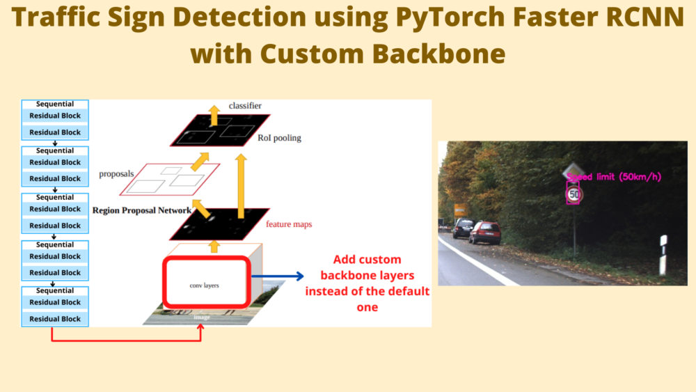
This post is going to be really exciting from a practical standpoint in deep learning and object detection. In the field of deep learning and computer vision, we regularly use pretrained object detection models and fine-tune them on our own dataset. Most of the time, we use these object detection models as it is without any modification except for the number of classes. But sometimes, slight changes in the architecture can produce exciting results. Maybe using a different custom backbone will give us better FPS during inference. Here, we are going to do something similar. In this post, we will carry out traffic sign detection using PyTorch Faster RCNN model with a custom backbone.
This is the last post in the traffic sign recognition and detection series:
- Traffic Sign Recognition using PyTorch and Deep Learning
- Traffic Sign Detection using PyTorch and Pretrained Faster RCNN Model
- Using Any Torchvision Pretrained Model as Backbone for PyTorch Faster RCNN
- Traffic Sign Recognition using Custom Image Classification Model in PyTorch
- Traffic Sign Detection using PyTorch Faster RCNN with Custom Backbone
We have covered a lot in this series till now. Starting from classification and detection using pretrained models, to switching backbones for Faster RCNN from Torchvision, to even using our own custom residual neural network for classification.
In this post, we will use the same custom residual neural network architecture as the backbone for PyTorch Faster RCNN. There are a lot of details that we will cover shortly. Although switching the backbone is an easy task, preparing the backbone is not as straightforward as it may seem. There are advantages and disadvantages to it and we will discuss them all here.
Topics to Cover
Let’s check out the topics we will cover in traffic sign detection using PyTorch Faster RCNN with Custom Backbone.
- We will start with a very short discussion of the dataset. We already covered the GTSDB dataset in detail in the previous posts.
- Then we will move over to the pretraining techniques of the custom residual neural network. This will be a very important section.
- Next, we will cover the preparation of the dataset briefly as it was already covered in detail in one of the previous posts in the series.
- The traffic sign detection training and detection code will be very similar to the previous posts in the series. However, well discuss all the little changes before we start the training. This includes the new new PyTorch Faster RCNN model with the custom backbone.
- After training, we will carry out inference on the both images and videos.
- Finally, we will discuss some of the advantages and disadvanted of using the PyTorch Faster RCNN model with custom backbone.
Note: In this post, we will mainly focus on the idea of using a custom backbone with the PyTorch Faster RCNN model. We will not focus on the accuracy of the trained model to a great extent. There are good reasons for this and we will discuss them in their respective sections.
The GTSDB Dataset
We will use the same GTSDB dataset that we have been using for the detection posts in this series. We have covered the details here.
The following is one of the images from the dataset with the ground truth annotations.
If you are new to this series of posts, then you may need to download the dataset.
You can visit the link to download them or click on the following direct download links:
For the training of the neural network on your own system, you will need a few more files. We will discuss them shortly and also downloading the zip file for this post will give access to them.
The Directory Structure
The directory structure will remain very similar to the previous detection posts. There are a few additional files that we will discuss here.
├── inference_outputs
│   └── videos
│       └── video_1_trimmed_1.mp4
├── input
│   ├── inference_data
│   │   ├── video_1.mp4
│   │   └── video_1_trimmed_1.mp4
│   ├── pretrained_voc_weights
│   │   └── last_model_state.pth
│   ├── TestIJCNN2013
│   │   └── TestIJCNN2013Download [301 entries exceeds filelimit, not opening dir]
│   ├── TrainIJCNN2013 [646 entries exceeds filelimit, not opening dir]
│   ├── train_images [425 entries exceeds filelimit, not opening dir]
│   ├── train_xmls [425 entries exceeds filelimit, not opening dir]
│   ├── valid_images [81 entries exceeds filelimit, not opening dir]
│   ├── valid_xmls [81 entries exceeds filelimit, not opening dir]
│   ├── all_annots.csv
│   ├── classes_list.txt
│   ├── gt.txt
│   ├── MY_README.txt
│   ├── signnames.csv
│   ├── train.csv
│   └── valid.csv
├── outputs
│   ├── last_model.pth
│   └── train_loss.png
├── src
│   ├── models
│   │   ├── fasterrcnn_custom_resnet.py
│   │   ├── fasterrcnn_mobilenetv3_large_320_fpn.py
│   │   ├── fasterrcnn_mobilenetv3_large_fpn.py
│   │   ├── fasterrcnn_resnet18.py
│   │   ├── fasterrcnn_resnet50.py
│   │   ├── fasterrcnn_squeezenet1_0.py
│   │   └── fasterrcnn_squeezenet1_1.py
│   ├── torch_utils
│   │   ├── coco_eval.py
│   │   ├── coco_utils.py
│   │   ├── engine.py
│   │   ├── README.md
│   │   └── utils.py
│   ├── config.py
│   ├── csv_to_xml.py
│   ├── custom_utils.py
│   ├── datasets.py
│   ├── inference.py
│   ├── inference_video.py
│   ├── split_train_valid.py
│   ├── train.py
│   └── txt_to_csv.py
Let’s go over the important bits in the above directory structure.
- Apart from the regular training and test data in the
inputdirectory, we also have apretrained_voc_weightssubdirectory. This contains the model weights which has been pretrained on the PASCAL VOC dataset. We will discuss the details in the next section of this post. All other files remain exactly the same. - Now, coming to
src/modelsdirectory. This time, along with all the previous Faster RCNN models, we have the newfasterrcnn_custom_resnet.py. This uses the same classification model as backbone that we use for traffic sign recognition in the last tutorial. We will discuss the details of this file before starting the training.
There are no other new files apart from the above two. However, there are a few other changes in the content of some of the files that we will discuss in the respective sections.
Apart from the GTSDB dataset (link provided in the previous section), you will get access to all other files and folders when downloading the zip file for this post.
Libraries and Frameworks
This series uses PyTorch 1.10.0 and Torchvision 0.11.1. Newer versions should also work but older versions may cause issues. And you will need Albumentations for image augmentations.
- Install the latest version of PyTorch from here.
- Install the latest version of Albumentations from here.
Pretraining Techniques for the PyTorch Faster RCNN Model with Custom Backbone
We know that training object detection model from scratch is difficult. On top of that, we have two other difficulties here.
- The custom residual neural network that we are using from the last tutorial is very small. Less than 1.3 million parameters.
- We don’t have have a lot of training images in our dataset. There are only 425 training images.
For that reason, just creating the Faster RCNN model with the custom backbone and directly training it on the GTSDB dataset won’t help. In fact, from experiments, I found that the model was able to reach only around 2% mAP.
Therefore, I used a bunch of pretraining techniques for both, the custom residual neural network backbone, and the custom Faster RCNN model as well.
However, all these pretraining experiments were constraints to the computation power that I had access to. All the pretraining experiments were done on a machine with a single 10 GB RTX 3080 GPU.
Let’s discuss them.
Pretraining of the Custom Residual Neural Network Classification Model
It is general practice to pretrain classification models on the ImageNet dataset before using the features as a backbone for an object detection model. However, doing that on a single GPU is immensely time-consuming and did not seem very practical to do for a blog post where the objective is learning the techniques.
So, I trained it on the Tiny ImageNet dataset which contains 100000 training and 10000 validation images with 200 classes. You can find all the details here.
Training configurations and results:
- The model was trained for 90 epochs with SGD optimizer.
- Image augmentation like random flipping, random rotation, color jitter, and affine transformations were also used.
- By the end of 90 epochs, the model was able to achieve top-1 accuracy of 46.7% and top-5 accuracy of 73.23%. This was the best epoch and we further use these weights for object detection pretraining.
Pretraining of the Faster RCNN with Custom Backbone for Object Detection
We use the above-obtained weights and use the model features for pretraining the Faster RCNN model on the PASCAL VOC dataset. The model training set consisted of VOC 2012 and VOC 2007 trainval images. The 2007 test set was used as the validation set. This was perhaps the longest phase of the pretraining.
Training configurations and results:
- First, the model was trained for 90 epochs on PASCAL VOC 2007 + 2012 trainval dataset without any augmentations to learn the general features of the dataset. By the end of 90 epochs, the mAP for 0.5 IoU was 41.6%.
- We again use the above detection trained weights and continue training for another 90 epochs. This time though, we use augmentations like blur, motion blur, random brightness and contast, color jitter, random gamma, and random fog. By the end of 90 epochs, we had a model with an mAP of 45.5% at 0.5 IoU. This may not seem much, but considering the difficulty of the dataset, this is a good improvement.
For all the detection training, Cosine Annealing with Warm Restarts learning rate scheduler was used. The restart period was 25 epochs.
As we have this trained model now, we will load the weights after creating the Faster RCNN model with the custom backbone. Hopefully, now our very small and naive model has learned some general features and will perform better on the GTSDB dataset. But as we will see further, everything is not just as simple or straightforward.
Preparing the Dataset
Please follow the Dataset Preprocessing and Creating XML Files section in this post to prepare the dataset.
Else, you can directly execute the following commands from the src directory to prepare the dataset.
python txt_to_csv.py
python split_train_valid.py
python csv_to_xml.py
Traffic Sign Detection using PyTorch Faster RCNN with Custom Backbone
Here onward, we will discuss any coding-related points before we can start the training. This includes the custom model file, changes to the augmentations, and a few small changes to the executable training script.
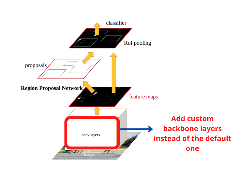
The Faster RCNN Model with Custom Backbone
The most important file in this post is the fasterrcnn_custom_resnet.py inside src/models.
Before executing the training script, first, we will discuss the new Faster RCNN model file.
The file contains the custom residual network definition first (that we covered in the last post), and then the function to create the final Faster RCNN model. For the sake of brevity, we are skipping the import statements and the classification model definition. Let’s focus on the final create_model function to create the Faster RCNN object detection model.
If you remember, our custom residual neural network had 5 Sequential layer blocks, each containing 2 residual blocks.
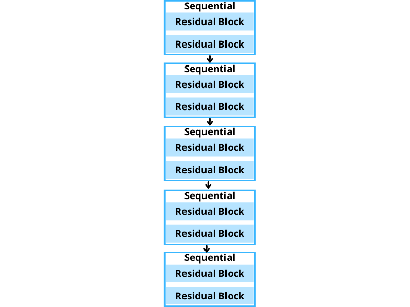
For that reason, it will be very simple to extract the feature from these 5 blocks. Let’s take a look at the code.
"""
Classification model definition above this.
"""

def create_model(num_classes):
    custom_resnet = CustomResNet(num_classes=10)
    block1 = custom_resnet.block1
    block2 = custom_resnet.block2
    block3 = custom_resnet.block3
    block4 = custom_resnet.block4
    block5 = custom_resnet.block5

    backbone = nn.Sequential(
        block1, block2, block3, block4, block5
    )

    backbone.out_channels = 256

    # Generate anchors using the RPN. Here, we are using 5x3 anchors.
    # Meaning, anchors with 5 different sizes and 3 different aspect
    # ratios.
    anchor_generator = AnchorGenerator(
        sizes=((32, 64, 128, 256, 512),),
        aspect_ratios=((0.5, 1.0, 2.0),)
    )

    # Feature maps to perform RoI cropping.
    # If backbone returns a Tensor, `featmap_names` is expected to
    # be [0]. We can choose which feature maps to use.
    roi_pooler = torchvision.ops.MultiScaleRoIAlign(
        featmap_names=['0'],
        output_size=7,
        sampling_ratio=2
    )

    # Pascal VOC Faster RCNN model.
    model = FasterRCNN(
        backbone=backbone,
        num_classes=21,
        rpn_anchor_generator=anchor_generator,
        box_roi_pool=roi_pooler
    )

    # Load the PASCAL VOC pretrianed weights.
    print('Loading PASCAL VOC pretrained weights...')
    checkpoint = torch.load('../input/pretrained_voc_weights/last_model_state.pth')
    model.load_state_dict(checkpoint['model_state_dict'])

    # Replace the Faster RCNN head with required class number. Final model.
    model = FasterRCNN(
        backbone=backbone,
        num_classes=num_classes,
        rpn_anchor_generator=anchor_generator,
        box_roi_pool=roi_pooler
    )

    return model
As we can see, from lines 7 to 11, we are extracting the 5 blocks of the backbone. Then we are adding all of them to a Sequential block on line 13. The output channels in the last convolutional layer of the classification model were 256. For that reason, here backbone.out_channels is also 256.
Then we create the anchor_generator and roi_pooler. The next important point to note here is on line 37. First, we create a Faster RCNN model with 21 classes. This is to have the exact model we had for training on the PASCAL VOC dataset so that we can load the trained models. We are loading the checkpoint and model weights on lines 46 and 47 respectively.
Finally, on line 50, we create the Faster RCNN model that we need for the GTSDB training with the proper number of classes.
This is all we need for the Faster RCNN model. This was not difficult even with a custom backbone.
Changes in the Augmentations
As we are training a very simple model here, although pretrained on the PASCAL VOC dataset, is not a very powerful one. Adding too many augmentations as we had before may make the training dataset very difficult. For that reason, we have removed all the augmentation from the get_train_transform() function in the custom_utils.py file apart from the tensor conversion.
Training Results
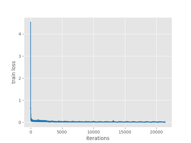
Let’s start with the training of the model. The following are the training configurations:
- Trained for 200 epochs.
- We use Cosine Annealing with Warm Restarts Scheduling with a restart period of 10 epochs.
Open the terminal/command line in the src directory and execute the following command.
python train.py
The following is the truncated output from the terminal.
python train.py
Number of training samples: 425
Number of validation samples: 81

Loading PASCAL VOC pretrained weights...
17,611,975 total parameters.
17,611,975 training parameters.

Epoch     0: adjusting learning rate of group 0 to 1.0000e-04.
Epoch: [0]  [  0/107]  eta: 0:01:15  lr: 0.000001  loss: 4.5259 (4.5259)  loss_classifier: 3.8298 (3.8298)  loss_box_reg: 0.0001 (0.0001)  loss_objectness: 0.6919 (0.6919)  loss_rpn_box_reg: 0.0041 (0.0041)  time: 0.7030  data: 0.1766  max mem: 568
Epoch: [0]  [100/107]  eta: 0:00:00  lr: 0.000101  loss: 0.0818 (0.4256)  loss_classifier: 0.0354 (0.2036)  loss_box_reg: 0.0024 (0.0047)  loss_objectness: 0.0338 (0.2090)  loss_rpn_box_reg: 0.0077 (0.0084)  time: 0.0527  data: 0.0050  max mem: 769
Epoch: [0]  [106/107]  eta: 0:00:00  lr: 0.000100  loss: 0.0728 (0.4057)  loss_classifier: 0.0332 (0.1940)  loss_box_reg: 0.0029 (0.0045)  loss_objectness: 0.0309 (0.1989)  loss_rpn_box_reg: 0.0061 (0.0083)  time: 0.0498  data: 0.0049  max mem: 769
Epoch: [0] Total time: 0:00:06 (0.0594 s / it)
creating index...
index created!
Test:  [ 0/21]  eta: 0:00:03  model_time: 0.0183 (0.0183)  evaluator_time: 0.0018 (0.0018)  time: 0.1738  data: 0.1492  max mem: 769
Test:  [20/21]  eta: 0:00:00  model_time: 0.0130 (0.0131)  evaluator_time: 0.0011 (0.0012)  time: 0.0212  data: 0.0054  max mem: 769
Test: Total time: 0:00:00 (0.0305 s / it)
Averaged stats: model_time: 0.0130 (0.0131)  evaluator_time: 0.0011 (0.0012)
Accumulating evaluation results...
DONE (t=0.04s).
IoU metric: bbox
 Average Precision  (AP) @[ IoU=0.50:0.95 | area=   all | maxDets=100 ] = 0.000
 Average Precision  (AP) @[ IoU=0.50      | area=   all | maxDets=100 ] = 0.000
 Average Precision  (AP) @[ IoU=0.75      | area=   all | maxDets=100 ] = 0.000
 Average Precision  (AP) @[ IoU=0.50:0.95 | area= small | maxDets=100 ] = 0.000
 Average Precision  (AP) @[ IoU=0.50:0.95 | area=medium | maxDets=100 ] = 0.000
 Average Precision  (AP) @[ IoU=0.50:0.95 | area= large | maxDets=100 ] = -1.000
 Average Recall     (AR) @[ IoU=0.50:0.95 | area=   all | maxDets=  1 ] = 0.000
 Average Recall     (AR) @[ IoU=0.50:0.95 | area=   all | maxDets= 10 ] = 0.000
 Average Recall     (AR) @[ IoU=0.50:0.95 | area=   all | maxDets=100 ] = 0.000
 Average Recall     (AR) @[ IoU=0.50:0.95 | area= small | maxDets=100 ] = 0.000
 Average Recall     (AR) @[ IoU=0.50:0.95 | area=medium | maxDets=100 ] = 0.000
 Average Recall     (AR) @[ IoU=0.50:0.95 | area= large | maxDets=100 ] = -1.000
SAVING PLOTS COMPLETE...
...
Epoch: [199]  [  0/107]  eta: 0:00:27  lr: 0.000010  loss: 0.0068 (0.0068)  loss_classifier: 0.0042 (0.0042)  loss_box_reg: 0.0025 (0.0025)  loss_objectness: 0.0000 (0.0000)  loss_rpn_box_reg: 0.0001 (0.0001)  time: 0.2603  data: 0.2039  max mem: 769
Epoch: [199]  [100/107]  eta: 0:00:00  lr: 0.000002  loss: 0.0067 (0.0074)  loss_classifier: 0.0019 (0.0021)  loss_box_reg: 0.0047 (0.0053)  loss_objectness: 0.0000 (0.0000)  loss_rpn_box_reg: 0.0000 (0.0001)  time: 0.0496  data: 0.0054  max mem: 769
Epoch: [199]  [106/107]  eta: 0:00:00  lr: 0.000002  loss: 0.0071 (0.0074)  loss_classifier: 0.0021 (0.0021)  loss_box_reg: 0.0047 (0.0052)  loss_objectness: 0.0000 (0.0000)  loss_rpn_box_reg: 0.0000 (0.0001)  time: 0.0483  data: 0.0052  max mem: 769
Epoch: [199] Total time: 0:00:05 (0.0529 s / it)
creating index...
index created!
Test:  [ 0/21]  eta: 0:00:04  model_time: 0.0159 (0.0159)  evaluator_time: 0.0021 (0.0021)  time: 0.2251  data: 0.2035  max mem: 769
Test:  [20/21]  eta: 0:00:00  model_time: 0.0124 (0.0127)  evaluator_time: 0.0018 (0.0019)  time: 0.0215  data: 0.0052  max mem: 769
Test: Total time: 0:00:00 (0.0339 s / it)
Averaged stats: model_time: 0.0124 (0.0127)  evaluator_time: 0.0018 (0.0019)
Accumulating evaluation results...
DONE (t=0.05s).
IoU metric: bbox
 Average Precision  (AP) @[ IoU=0.50:0.95 | area=   all | maxDets=100 ] = 0.024
 Average Precision  (AP) @[ IoU=0.50      | area=   all | maxDets=100 ] = 0.062
 Average Precision  (AP) @[ IoU=0.75      | area=   all | maxDets=100 ] = 0.000
 Average Precision  (AP) @[ IoU=0.50:0.95 | area= small | maxDets=100 ] = 0.024
 Average Precision  (AP) @[ IoU=0.50:0.95 | area=medium | maxDets=100 ] = 0.000
 Average Precision  (AP) @[ IoU=0.50:0.95 | area= large | maxDets=100 ] = -1.000
 Average Recall     (AR) @[ IoU=0.50:0.95 | area=   all | maxDets=  1 ] = 0.027
 Average Recall     (AR) @[ IoU=0.50:0.95 | area=   all | maxDets= 10 ] = 0.032
 Average Recall     (AR) @[ IoU=0.50:0.95 | area=   all | maxDets=100 ] = 0.032
 Average Recall     (AR) @[ IoU=0.50:0.95 | area= small | maxDets=100 ] = 0.032
 Average Recall     (AR) @[ IoU=0.50:0.95 | area=medium | maxDets=100 ] = 0.000
 Average Recall     (AR) @[ IoU=0.50:0.95 | area= large | maxDets=100 ] = -1.000
SAVING PLOTS COMPLETE...
As you see, even with pretained PASVAL VOC weights, the model was not able to achieve a very high mAP. In the last epoch, mAP for IoU=0.50 is only 6.2%. And it reached around 6.5% somewhere in-between. This shows how much difficult it is to train an object detection model with a custom backbone on a small dataset that has not been pretrained on the MS COCO dataset.
It is very difficult to improve the model any further without proper pretraining. For now, let’s see what kind of results we get while inferencing.
Inference on Images using PyTorch Faster RCNN Model with Custom Backbone
While inferencing, we will use a reduced threshold of 0.3 this time.
python inference.py --input ../input/TestIJCNN2013/TestIJCNN2013Download --threshold 0.3
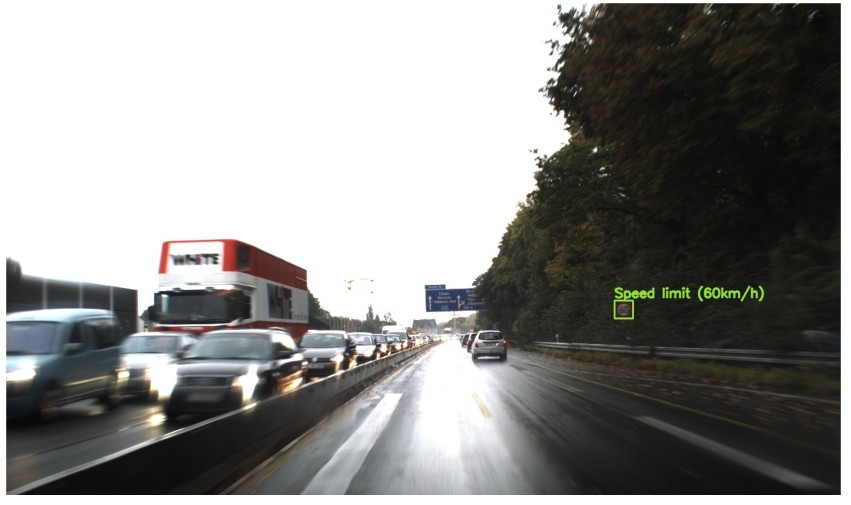
On an RTX 3080 GPU, the model was giving over 130 FPS which is really great. This is the highest FPS that we have till now in this series. Let’s take a look at some of the successful predictions.
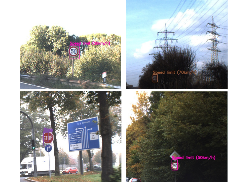
The above figure shows that the model is able to predict some of the speed signs, and a few easier signs correctly.
Now, some of the missed/improper and incorrect predictions.
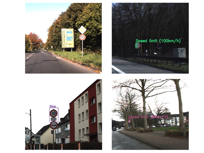
As we can see, it is missing a lot, even some of the obvious ones.
Inference on Video
Before making any further conclusions, let’s take a look at the video predictions.
python inference_video.py --input ../input/inference_data/video_1_trimmed_1.mp4 --threshold 0.3
The above video is not from the dataset and therefore, is particularly difficult for the model. Still, in the previous posts, other models were able to perform fairly well on this one too. Here, the model is missing almost all except a very few simple ones, and that too when the sign is very close to the screen only.
A Few Takeaways
This project may seem like a failure on many fronts but it actually teaches a lot. When carrying out all the experiments, pretraining, and tracking everything down, I personally learned a lot.
- The first lesson, creating custom models (especially for object detection) is not that easy.
- Secondly, the pretraining needed for any new and custom model is not a simple job to carry out. I had decent compute resources. With that, a fairly simple image classification pretraining, and somewhat advanced PASCAL VOC pretraining was possible. These two experiments took nearly three days. Not to mention collecting data, preparing it, and writing the code, which takes even more time.
- Even then, when trying to fine-tune our model, it did not perform very well. Although we got the highest FPS for detection than any other model in this series. The detections were simply not a match even for the SqueezeNet models that we covered in the previous posts.
- Deep learning libraries and frameworks like PyTorch and TensorFlow make our life a lot easier by providing so many tools and pretrained models. And that’s why we are able to train so many models on our own dataset. It was pretty evident from the previous posts in the series.
After these experiments, we should be able to respect the researchers and developers even more who provides us with so many great models and tools to use for free.
Summary and Conclusion
In this post, we tried to train a custom PyTorch Faster RCNN model. The detections results were not good of course. This shows how difficult it can be to create and train an object detection model on a small dataset from scratch is. This also marks the end of the traffic sign recognition and detection series. Although a failure on the results front, hopefully, this post and the entire series were a good learning experience for you.
If you have any doubts, thoughts, or suggestions, please leave them in the comment section. I will surely address them.
You can contact me using the Contact section. You can also find me on LinkedIn, and X.
