Simple Facial Keypoint Detection using TensorFlow and Keras

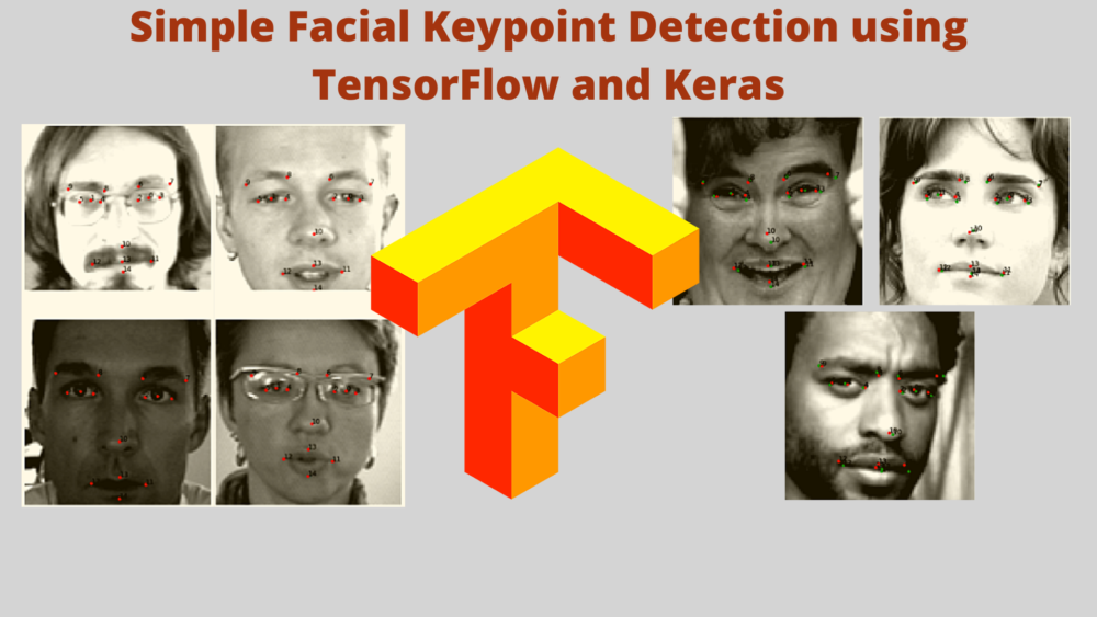
In computer vision, face-related applications cover a major area. With deep learning leading a lot of computer vision based applications, it is indirectly leading the face-related applications as well. Starting from face recognition, to facial keypoint detection, to even security and surveillance applications. All of these tend to use deep learning and computer vision in some way or the other. And for sure, convolutional neural networks are a leading architecture for all of these. As such, it is good to have some knowledge of applying deep learning and computer vision face-related applications. With that in mind, we will solve a simple problem in this tutorial. We will cover a very simple training pipeline for facial keypoint detection using TensorFlow and Keras.

This post will cover very basic and simple training for facial keypoint detection. As we will be using TensorFlow and Keras as the frameworks of choice, our work will become even easier. Although this is the starting point, in future posts, we will cover more advanced training along the same line.

Let’s take a look at the points that we will cover in this post.

• We will start off, with a small discussion about the need for facial keypoint detection.
• Next, we will discuss the dataset that we will use in this tutorial.
• Then, we will discuss the directory structure, and all the library/framework-related dependencies and versions.
• Following that, we will move on to the coding and training part of the tutorial.
• After training and saving the model, we will also carry predictions on the validation and test images.
• In the end, we will discuss what we learned and what are some of the possible drawbacks of the approach that we follow in this tutorial.

Note…

If you are more of a PyTorch favoring deep learning practitioner, then I have a similar training pipeline on the same dataset with PyTorch here.

Importance of Facial Keypoint Detection

By now, we have established that it is better to have some knowledge of facial keypoint detection and face applications in general. But what are some of the real-life applications of facial keypoint detection and computer vision-aided face applications? Let’s try to lay out some points here.

• Security and surveillance: This is perhaps one of the best use cases for face recognition and facial landmark detection. Deep learning and computer vision models deployed on edge devices can help identify threats. They try to recognize persons on security cameras. This can help prevent a number of crimes that otherwise may be unavoidable.
• Filters on smartphone apps: This is one of the fun use cases of facial landmark detection. And one of the best known out there are the Snapchat filters which work very well even with faces that are constantly moving. All of this is possible because of a combination of face detection and facial keypoint detection.
• Securing devices: Locking and unlocking devices is also aided by facial keypoint detection. One of the common ones that many of us may have used is unlocking our smartphones via face recognition. This is also a combination of face detection, face recognition, and facial keypoint or landmark detection.

The above cover only a few applications. But there are numerous others. In fact, there are people in the computer vision and deep learning industry who have sole expertise in the face detection, recognition, and face-related applications field.

It is pretty evident that it is always a combination of technologies that goes into the final applications. Here, in this tutorial, we will start with simple facial keypoint detection using TensorFlow and Keras.

The Facial Keypoint Dataset

In this tutorial, to start the simple facial keypoint detection using TensorFlow and Keras, we will use this dataset.

This Kaggle dataset is from the Facial Keypoints Detection competition. Here, we have to detect the location of keypoints on face images.

Interestingly, the dataset does not contain any raw image files. All the dataset is present in two CSV files. After downloading and extracting the dataset, you will get the training.csv and test.csv files. The training.csv file contains the data in the following format.

left_eye_center_x	left_eye_center_y	right_eye_center_x	right_eye_center_y ... Image
66.033564	        39.002274	         30.227008	        36.421678	       238 2236 237 ...

There are a total of 31 columns. The first 30 columns contain the keypoint coordinates for the faces. Now, take note that the columns are in order of x and y coordinate for each part of the face. For example, first left_eye_center_x (x-coordinate) and left_eye_center_y (y-coordinate) for the left eye. Then for the right eye, and so on. The final column is the Image column containing all the pixel values for a 96×96 resolution grayscale image. To use it properly, we will have to reshape these values later on. If you open the CSV file, you will have a pretty good idea about it.

After extracting the dataset, you may find two other CSV files as well, but we don’t need them. It is also worthwhile to keep in mind that the test.csv file only contains the image information, as that is to be used for the competition submission. We will test our trained model on images in this file later on.

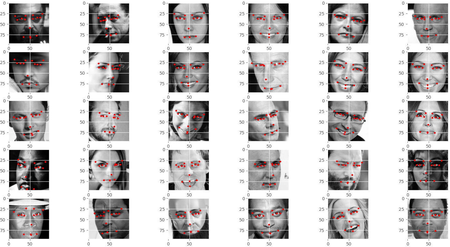
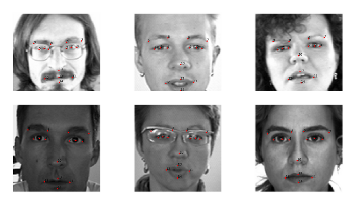
For now, let’s take a look at some ground truth images that we can extract from the training.csv file.

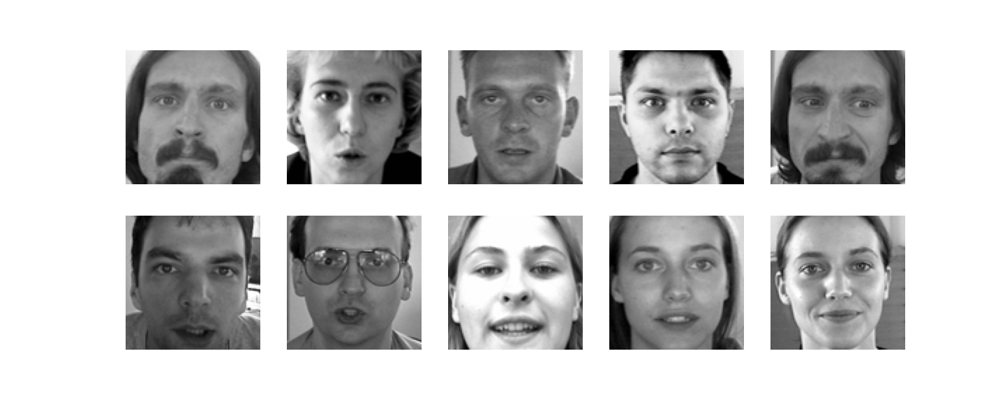
As you can see, all the images are in grayscale format.

The following figure shows the same images but with the keypoints.

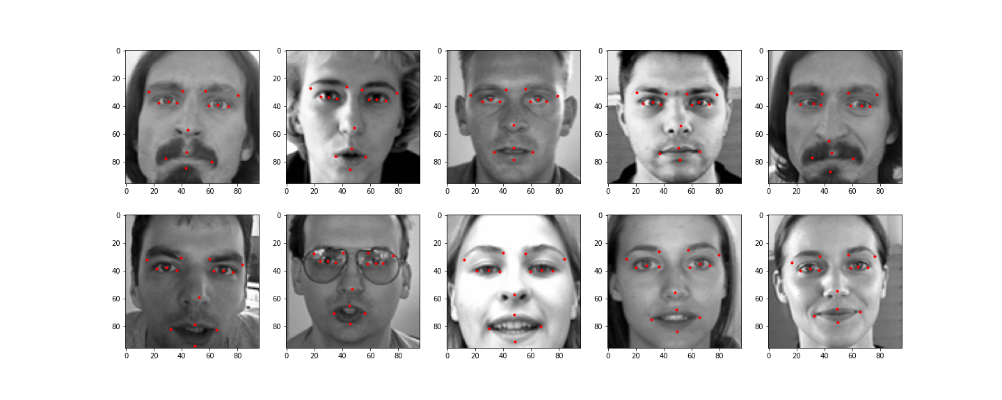
We can see the fifteen keypoints on the faces.

An Important Note About the Dataset

If you open the training.csv file, you will find that there are more than 7000 instances. But a lot of them are missing the information in some or all of the columns. And for obvious reasons, we cannot directly read the dataset from this CSV file and just feed it to our neural network. We need to clean this up. We will get to know more about this step while preparing the dataset in the coding section.

For now, please head over to the competition page and download the dataset. In the next section, we will see how to extract and structure the directory for the input files and other Python files as well.

Directory Structure

The following block shows the directory structure for all the files/folders.

├── input
│   ├── IdLookupTable.csv
│   ├── SampleSubmission.csv
│   ├── test.csv
│   └── training.csv
├── outputs
│   ├── saved_model
│   │   ├── assets
│   │   ├── variables
│   │   │   ├── variables.data-00000-of-00001
│   │   │   └── variables.index
│   │   ├── keras_metadata.pb
│   │   └── saved_model.pb
│   ├── test_results [1783 entries exceeds filelimit, not opening dir]
│   ├── validation_results [416 entries exceeds filelimit, not opening dir]
│   └── loss.png
├── src
│   ├── config.py
│   ├── dataset.py
│   ├── evaluate_and_test.py
│   ├── model.py
│   ├── train.py
│   └── utils.py

Let’s go over the important files/directories.

• The input directory contains all the CSV files after extracting the dataset. Make sure to have your own structure like this as well.
• The outputs directory will hold the saved TensorFlow model after training, and also the test and validation image results. It will also contain the loss graph that we obtain from training.
• And the src directory contains all the Python files that we need for facial keypoint detection using TensorFlow and Keras. We will discuss these in the coding section.

Apart from the files in the input directory, you will get access to all others while downloading the zip file for this tutorial.

TensorFlow and Keras Versions

All the code in this tutorial has been developed using TensorFlow 2.7.0 and Keras 2.7.0. Be sure to have the same version or at least TensorFlow version 2.6.0. With the latest versions of TensorFlow 2.x, Keras will be automatically installed, so you don’t need to install it manually.

Simple Facial Keypoint Detection using TensorFlow and Keras

Let’s start with the coding part of this tutorial. We will cover each of the Python files in the src directory in the following order:

• config.py
• utils.py
• dataset.py
• model.py
• train.py

The above scripts will take us till the end of training the TensorFlow deep learning model on the facial keypoints dataset. Then we will use the evaluate_and_test.py to carry out inference on the validation and test set.

The Configuration File

The configuration Python file contains some of the general configurations we need for training and testing. They are the root data path, the learning parameters, and the train/test split percentage.

The following code will go into the config.py file.

# Input root path.
ROOT_PATH = '../input'

# Learning parameters.
BATCH_SIZE = 32
LR = 0.001
EPOCHS = 300
IMGAE_RESIZE = 96

# Train/test split.
TEST_SPLIT = 0.2

# Show dataset keypoint plot (executing `dataset.py`).
SHOW_DATASET_PLOT = True

As we can see, we have set up all the required configurations here. We can use these throughout the training and inference pipeline very easily. The only odd one here is the SHOW_DATASET_PLOT. If this is True, and we execute dataset.py from the terminal, then it will show us a plot of the faces with the ground truth facial keypoints. We will get into more details about these while writing the dataset preparation code.

Helper Functions and Utilities

Even a simple deep learning training pipeline will require some utility scripts and helper functions. And it is always better to have them in a separate module from the beginning and not in the same executable training script. This will ensure we can import them whenever we need them without cluttering other parts of the code.

Here, we will write four helper functions. And all of them will go into the utils.py file.

Helper Function to Plot Ground Truth and Predicted Keypoints on the Validation Data

Starting with the imports and the first helper function.

import matplotlib.pyplot as plt
import numpy as np
import os

plt.style.use('ggplot')

def evaluation_keypoints_plot(
    image, outputs, orig_keypoints, save_path
):
    """
    This function plots the regressed (predicted) keypoints from all the 
    evalutaion images.
    """
    output_keypoint = outputs.reshape(-1, 2)
    orig_keypoint = orig_keypoints.reshape(-1, 2)
    image = image.reshape(96, 96)
    plt.style.use('default')
    plt.imshow(image, cmap='gray')
    plt.axis('off')
    for p in range(output_keypoint.shape[0]):
        plt.plot(output_keypoint[p, 0], output_keypoint[p, 1], 'r.')
        plt.text(output_keypoint[p, 0], output_keypoint[p, 1], f"{p}")
        plt.plot(orig_keypoint[p, 0], orig_keypoint[p, 1], 'g.')
        plt.text(orig_keypoint[p, 0], orig_keypoint[p, 1], f"{p}")

    plt.savefig(save_path)
    plt.close() 

We have the evaluation_keypoints_plot function in the above code block. It accepts the image, the outputs keypoints, the original keypoints (orig_keypoints), and the save_path string to save the image. This will plot the ground truth keypoints from the validation data and the predicted (regressed) keypoints on the current validation image. Note that the image we pass has dimension (HxWx1). So, we need to reshape it before we can plot it using Matplotlib.

After plotting the keypoints, we save them to disk for later analysis. Taking a look at the images will give us a good idea of how well the TensorFlow deep learning model has learned.

Helper Function to Plot Predicted Keypoints from the Test Data

After training, we will also predict the keypoints on the image data present in the test.csv file. Let’s write a helper function for that as well, that will be very similar to the above one, except for the ground truth data.

def test_keypoints_plot(image, outputs, save_path):
    """
    This function plots the keypoints for the outputs and images
    from the `test.csv` file.
    """
    output_keypoint = outputs.reshape(-1, 2)
    image = image.reshape(96, 96)
    plt.style.use('default')
    plt.imshow(image, cmap='gray')
    plt.axis('off')
    for p in range(output_keypoint.shape[0]):
        plt.plot(output_keypoint[p, 0], output_keypoint[p, 1], 'r.')
        plt.text(output_keypoint[p, 0], output_keypoint[p, 1], f"{p}")

    plt.savefig(save_path)
    plt.close()

The above function only plots the regressed keypoints for the test images as the test data does not contain any ground truth data.

Helper Function to Plot Image and Keypoints from Sequence Data

Further in the coding part, we will write our custom Sequence dataset class to create training and validation datasets. Let’s write a function so that we can visualize the images and ground truth keypoints from the datasets.

def dataset_keypoints_plot(data):
    """
    This function shows the image faces and keypoint plots that the model
    will actually see. This is a good way to validate that our dataset is in
    fact correct and the faces align with the keypoint features. The plot 
    will be show if you execute `dataset.py`.
    """
    plt.figure(figsize=(20, 40))
    for i in range(30):
        img = data[0][0][i]
        img = np.array(img, dtype='float32')
        img = img.reshape(96, 96)
        plt.subplot(5, 6, i+1)
        plt.imshow(img, cmap='gray')
        keypoints = data[0][1][i]
        keypoints = keypoints.reshape(-1, 2)
        for j in range(len(keypoints)):
            plt.plot(keypoints[j, 0], keypoints[j, 1], 'r.')
    plt.show()
    plt.close()

The dataset_keypoints_plot accepts a Sequence data object and plots 30 faces with their keypoints. After writing the code in dataset.py further on, if we execute that file from the terminal, then the image will be plotted.

Helper Function to Plot the Loss

Now, we just have one more helper function. It is a simple one for plotting and saving the loss graphs to disk.

def save_plots(history):
    """
    Function to save the loss and accuracy plots to disk.
    """
    train_loss = history.history['loss']
    valid_loss = history.history['val_loss']
    # Loss plots.
    plt.figure(figsize=(12, 9))
    plt.plot(
        train_loss, color='orange', linestyle='-', 
        label='train loss'
    )
    plt.plot(
        valid_loss, color='red', linestyle='-', 
        label='validataion loss'
    )
    plt.xlabel('Epochs')
    plt.ylabel('Loss')
    plt.legend()
    plt.savefig(os.path.join(
        '..', 'outputs', 'loss.png'
    ))
    plt.show()

The save_plots accepts the training history object and saves the loss graph to disk.

Preparing the Dataset

Now, it’s time to complete one of the most important parts of the tutorial. Writing the code to prepare the dataset for facial keypoint detection using TensorFlow and Keras.

We will write the dataset preparation code in the dataset.py file.

First, let’s import all the modules and libraries.

import cv2
import pandas as pd
import numpy as np
import config
import utils

from tensorflow.keras.utils import Sequence
from tqdm import tqdm

resize = config.IMGAE_RESIZE

Along with all the required libraries, we are also importing our own config and utils modules. And you can see that we are defining the resize variable according to the configuration file. We will use the Sequence class to prepare our custom dataset loader here, as that will be much easier to manage given the format in which we have the data.

Cleaning and Splitting the Data

As we discussed earlier, there are more than 7000 rows of data available in the training CSV file. But a lot of them have missing values. We have to clean the data so that there are no errors when extracting the values. In this situation, there are two options. We either take the average of all the respective keypoint columns and fill them up in the missing columns. Or drop all the missing data rows altogether.

The first approach is a bit error-prone as there is no guarantee the average values of keypoints will satisfy well enough for all the images which are missing the values. There is a very high chance that the model may learn from the wrong data. For that reason, we will just drop those rows. Surely, we will have much fewer instances, but at least, all of them will be correct.

The following train_test_split function does two things:

• Cleans up the data by dropping all the rows with missing values.
• Splits the data into a train and validation set.

def train_test_split(csv_path, split):
    df_data = pd.read_csv(csv_path)
    # Drop all the rows with missing values.
    df_data = df_data.dropna()
    len_data = len(df_data)
    # Calculate the validation data sample length.
    valid_split = int(len_data * split)
    # Calculate the training data samples length.
    train_split = int(len_data - valid_split)
    training_samples = df_data.iloc[:train_split][:]
    valid_samples = df_data.iloc[-valid_split:][:]
    print(f"Training sample instances: {len(training_samples)}")
    print(f"Validation sample instances: {len(valid_samples)}")
    return training_samples, valid_samples

The above function accepts the CSV file path and the split ratio as parameters. After cleaning and splitting the data, it returns the training_samples and valid_samples data frames.

The Sequence Data Class

The next thing important thing here is to write a custom dataset using the Sequence class. We will not go into the details of the working of Sequence class here.

Let’s write the FaceKeypointDataset dataset here.

class FaceKeypointDataset(Sequence):
    def __init__(self, samples, batch_size):
        self.batch_size = batch_size
        self.data = samples
        # Get the image pixel column only.
        self.pixel_col = self.data.Image
        self.image_pixels = []
        for i in tqdm(range(len(self.data))):
            img = self.pixel_col.iloc[i].split(' ')
            self.image_pixels.append(img)

        self.images = np.array(self.image_pixels, dtype='float32')

    def __len__(self):
        return len(self.data) // self.batch_size
    
    def __getitem__(self, index):
        batch_images = self.images[index*self.batch_size:(index+1)*self.batch_size]
        batch_keypoints = self.data.iloc[index*self.batch_size:(index+1)*self.batch_size]
        final_images = []
        final_keypoints = []
        for j in range(self.batch_size):
            # Reshape the images into their original 96x96 dimensions.
            input_image = batch_images[j]
            image = input_image.reshape(96, 96)
            orig_w, orig_h = image.shape
            # Resize the image into `resize` defined above.
            image = cv2.resize(image, (resize, resize))
            # Again reshape to add grayscale channel format.
            image = image.reshape(resize, resize, 1)
            image = image / 255.0
            # Get the keypoints.
            keypoints = batch_keypoints.iloc[j][:30]
            keypoints = np.array(keypoints, dtype='float32')
            # Reshape the keypoints.
            keypoints = keypoints.reshape(-1, 2)
            # Rescale keypoints according to image resize.
            keypoints = keypoints * [resize / orig_w, resize / orig_h]
            keypoints = np.ravel(keypoints)
            final_images.append(image)
            final_keypoints.append(keypoints)
        final_images = np.array(final_images)
        final_keypoints = np.array(final_keypoints)
        return (final_images, final_keypoints)

It is mandatory to implement the __len__ and __getitem__ methods. Also, we need to ensure that the __getitem__ method returns a complete batch of data as per the batch_size passed on to the __init__ method.

The __init__ method above defines the batch_size, the data (either training or validation data frame), and stores all the image pixels in the images NumPy array.

As for the __getitem__ method, we return a batch of data in the form of final_images and final_keypoints NumPy arrays. Also, observe that we are resizing the images and adjusting the keypoints according to the resizing as per the resize parameter. This will ensure that we can freely choose any resizing factor in the configuration file.

Function to Return the Sequence Data

Now, we just need to finish up the final part of dataset preparation. We will write two simple functions. One to prepare the training and validation data frames, and the other to return the training and validation Sequence datasets.

# Get the training and validation data samples.
training_samples, valid_samples = train_test_split(
    f"{config.ROOT_PATH}/training.csv",
    config.TEST_SPLIT
)

def get_data():
    train_ds = FaceKeypointDataset(training_samples, batch_size=config.BATCH_SIZE)
    valid_ds = FaceKeypointDataset(valid_samples, batch_size=config.BATCH_SIZE)
    return train_ds, valid_ds

if __name__ == '__main__':
    # Show to show dataset keypoint plots if enabled in `config.py`.`
    if config.SHOW_DATASET_PLOT:
        _, valid_ds = get_data()
        utils.dataset_keypoints_plot(valid_ds)

The get_data function returns the training and validation datasets. Along with that, if we execute dataset.py itself, it will call the dataset_keypoints function from utils giving us the following output.

This completes our dataset preparation part.

The Neural Network Model

As you might have guessed by now, our neural network model is going to regress 30 keypoint values. Each of them corresponds to one set of coordinates from the 15 keypoint coordinate pairs from the faces. As such, it will have 30 units in the final Dense layer

Let’s write the model preparation code in model.py.

import tensorflow as tf

from tensorflow.keras import layers

def build_model(image_size):
    inputs = layers.Input(shape=(image_size[0], image_size[1], 1))
    # Conv => Activation => Pool blocks.
    x = layers.Conv2D(32, kernel_size=(5, 5))(inputs)
    x = layers.ReLU()(x)
    x = layers.MaxPool2D((2, 2))(x)

    x = layers.Conv2D(64, kernel_size=(3, 3))(x)
    x = layers.ReLU()(x)
    x = layers.MaxPool2D((2, 2))(x)

    x = layers.Conv2D(128, kernel_size=(3, 3))(x)
    x = layers.ReLU()(x)
    x = layers.MaxPool2D((2, 2))(x)

    x = layers.Conv2D(256, kernel_size=(3, 3))(x)
    x = layers.ReLU()(x)
    x = layers.MaxPool2D((2, 2))(x)
    
    x = layers.Conv2D(512, kernel_size=(3, 3))(x)
    x = layers.ReLU()(x)
    x = layers.MaxPool2D((2, 2))(x)
    
    # Linear layers.
    x = layers.GlobalAveragePooling2D()(x)
    x = layers.Dense(units=256)(x)
    x = layers.ReLU()(x)
    x = layers.Dense(units=30)(x)

    model = tf.keras.Model(inputs, outputs=x)
    return model

As you can see, instead of hardcoding the input image size, we are passing that as a parameter to the build_model function. This will ensure that the model code remains consistent with the image resizing in the confg.py file.

Apart from that, the model itself is pretty simple. First, we have a stacking of 2D convolutional layers, ReLU activation, and the 2D max-pooling layers.

The linear part of the network consists of two Dense layers, out of which the final one is the classification head with 30 units.

The Training Script

The training script is perhaps the simplest part of the entire pipeline. As we have defined almost all the components earlier, we just need to connect each of them and start the training.

We will write the training script code in the train.py file.

The following block contains the code for the entire training script.

from model import build_model
from dataset import get_data
from utils import save_plots

import config
import tensorflow as tf

# Model checkpoint callback.
model_ckpt = tf.keras.callbacks.ModelCheckpoint(
    filepath='../outputs/saved_model',
    monitor='val_loss',
    mode='auto',
    save_best_only=True
)

# Load the training and validation data.
train_ds, valid_ds = get_data()

# Build and compile the model.
model = build_model((config.IMGAE_RESIZE, config.IMGAE_RESIZE))
print(model.summary())
model.compile(
    optimizer=tf.keras.optimizers.Adam(learning_rate=config.LR), 
    loss=tf.keras.losses.MeanSquaredError(), 
)

# Train the model.
history = model.fit(
    train_ds,
    validation_data=valid_ds,
    epochs=config.EPOCHS,
    callbacks=[model_ckpt],
    workers=4, 
    use_multiprocessing=True
)

save_plots(history)

We import all the custom modules and tensorflow as well.

First, on line 9, we create a model checkpoint callback to save the best model according to the loss value.

Then on line 17, we load the training and validation datasets.

Next, we initialize the model and compile it. Observe that we are using only the MeanSquaredError loss here and no other metric. As this is a regression problem, it does not make much sense to have an accuracy metric here. Only a proper loss function should suffice.

Finally, we train the model with the callbacks and save the loss plots to disk.

Note: If you are on Windows OS, consider removing/commenting out the workers and use_multiprocessing arguments in the model.fit() method. Using these two arguments generally tends to freeze the training on Windows OS after the model initialization.

Executing train.py and Analyzing the Results

To run the training script, simply execute the following command in the terminal/command line within the src directory.

Note: We train here for 300 epochs. Even with moderately powerful hardware, it should not take more than 15-20 minutes to train.

python train.py 

The following block shows the truncated output from the terminal.

Training sample instances: 1712
Validation sample instances: 428
100%|███████████████████████████████████████████████████████████████████████████████████████████| 1712/1712 [00:00<00:00, 3709.54it/s]
100%|███████████████████████████████████████████████████████████████████████████████████████████| 428/428 [00:00<00:00, 4553.79it/s]
Model: "model"
_________________________________________________________________
 Layer (type)                Output Shape              Param #   
=================================================================
 input_1 (InputLayer)        [(None, 96, 96, 1)]       0         
                                                                 
 conv2d (Conv2D)             (None, 92, 92, 32)        832       
                                                                 
 re_lu (ReLU)                (None, 92, 92, 32)        0         
                                                                 
 max_pooling2d (MaxPooling2D  (None, 46, 46, 32)       0         
 )                                                               
                                                                 
 conv2d_1 (Conv2D)           (None, 44, 44, 64)        18496     
                                                                 
 re_lu_1 (ReLU)              (None, 44, 44, 64)        0         
                                                                 
 max_pooling2d_1 (MaxPooling  (None, 22, 22, 64)       0         
 2D)                                                             
                                                                 
 conv2d_2 (Conv2D)           (None, 20, 20, 128)       73856     
                                                                 
 re_lu_2 (ReLU)              (None, 20, 20, 128)       0         
                                                                 
 max_pooling2d_2 (MaxPooling  (None, 10, 10, 128)      0         
 2D)                                                             
                                                                 
 conv2d_3 (Conv2D)           (None, 8, 8, 256)         295168    
                                                                 
 re_lu_3 (ReLU)              (None, 8, 8, 256)         0         
                                                                 
 max_pooling2d_3 (MaxPooling  (None, 4, 4, 256)        0         
 2D)                                                             
                                                                 
 conv2d_4 (Conv2D)           (None, 2, 2, 512)         1180160   
                                                                 
 re_lu_4 (ReLU)              (None, 2, 2, 512)         0         
                                                                 
 max_pooling2d_4 (MaxPooling  (None, 1, 1, 512)        0         
 2D)                                                             
                                                                 
 global_average_pooling2d (G  (None, 512)              0         
 lobalAveragePooling2D)                                          
                                                                 
 dense (Dense)               (None, 256)               131328    
                                                                 
 re_lu_5 (ReLU)              (None, 256)               0         
                                                                 
 dense_1 (Dense)             (None, 30)                7710      
                                                                 
=================================================================
Total params: 1,707,550
Trainable params: 1,707,550
Non-trainable params: 0
_________________________________________________________________
Epoch 1/300
53/53 [==============================] - 4s 34ms/step - loss: 588.1769 - val_loss: 87.8794
Epoch 2/300
53/53 [==============================] - 2s 29ms/step - loss: 61.1080 - val_loss: 40.1440
Epoch 3/300
53/53 [==============================] - 2s 32ms/step - loss: 21.1378 - val_loss: 28.5753
Epoch 4/300
53/53 [==============================] - 2s 31ms/step - loss: 24.3583 - val_loss: 27.4814
Epoch 5/300
53/53 [==============================] - 2s 32ms/step - loss: 14.5680 - val_loss: 22.9587
...
Epoch 299/300
53/53 [==============================] - 1s 14ms/step - loss: 0.7052 - val_loss: 9.1143
Epoch 300/300
53/53 [==============================] - 1s 15ms/step - loss: 1.3051 - val_loss: 7.9403

By the end of the training, the training loss is hovering between 1.3 and 0.5 and the validation loss is somewhere around 7.9. Not very bad results considering such a simple model and simple training pipeline.

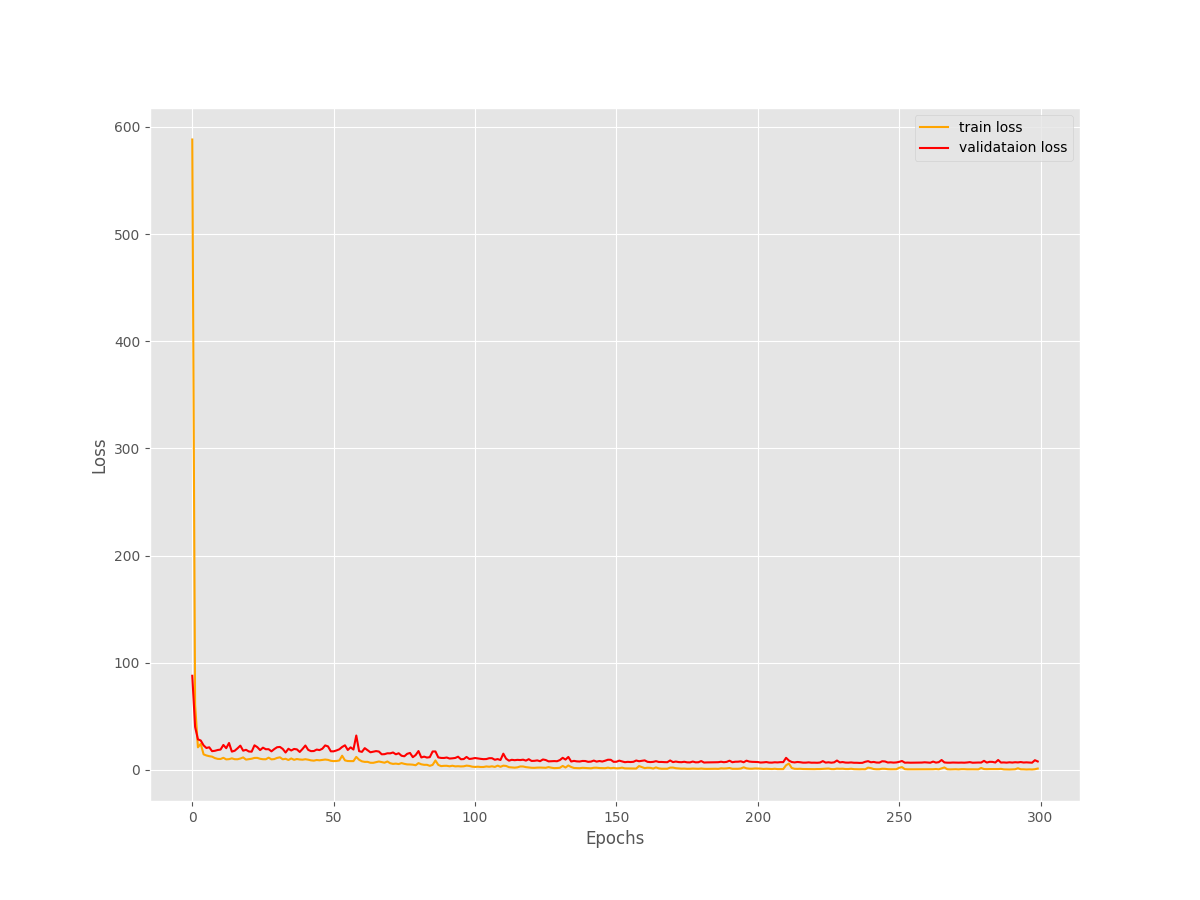
The loss plots do not show any sign of overfitting. Most probably, training for a few more epochs may give even better results.

Inference for Facial Keypoint Detection using TensorFlow and Keras using the Saved Model

After the training is complete, we have the trained model inside outputs/saved_model. We will use this trained model for two things:

• For predicting the keypoints in the validation set and checking out how well the predicted keypoints match the ground truth ones.
• For predicting the keypoints on the images in the test.csv file.

To accomplish the above two, we need to write a simple script.

The code for this will go into the evaluate_and_test.py file.

Let’s go over the code briefly. As usual, starting with the import statements. Along with that, let’s create the appropriate output directories to save the results, load the saved model, and the validation data as well.

"""
Script to evaluate the model on the validation dataset and
test it on the test dataset. Also, plot all the results and save them to disk.
"""

import tensorflow as tf
import os
import pandas as pd
import numpy as np

from dataset import get_data
from utils import evaluation_keypoints_plot, test_keypoints_plot
from tqdm import tqdm

# Create directory to save validation results.
validation_result_path = os.path.join('..', 'outputs', 'validation_results')
os.makedirs(os.path.join(validation_result_path), exist_ok=True)

# Create directory to save test results.
test_result_path = os.path.join('..', 'outputs', 'test_results')
os.makedirs(os.path.join(test_result_path), exist_ok=True)

model = tf.keras.models.load_model('../outputs/saved_model')
print(model.summary())

_, valid_ds = get_data()

The validation data images results will be saved in the validation_results directory and the test data images will be saved in the test_results directory.

The Evaluation and Test Functions

Next, we will write two functions. One for the validation dataset and one for predicting on the test.csv data.

def evaluate(valid_ds):
    # Get the results.
    results = model.predict(valid_ds)
    # Loop over the validation set and save the 
    # images and corresponding result plot to disk.
    counter = 0
    for i, batch in tqdm(enumerate(valid_ds), total=len(valid_ds)):
        for j, (image, keypoints) in enumerate(zip(batch[0], batch[1])):
            evaluation_keypoints_plot(
                image, results[counter], keypoints,
                save_path=os.path.join(validation_result_path, str(counter)+'.png')
            )
            counter += 1

def test(test_csv_path):
    """
    Function to predict on all images present in `test.csv` file
    """
    test_df = pd.read_csv(test_csv_path)
    images = test_df.Image
    for i in tqdm(range(len(images)), total=len(images)):
        image = images.iloc[i].split(' ')
        image = np.array(image, dtype=np.float32) / 255.
        image = image.reshape(96, 96)
        image = image.reshape(96, 96, 1)
        image_batch = np.expand_dims(image, axis=0)
        image_tensor = tf.convert_to_tensor(image_batch)
        outputs = model.predict(image_tensor)
        test_keypoints_plot(
            image, outputs, 
            save_path=os.path.join(test_result_path, str(i)+'.png')
        )

print('Evaluating...')
evaluate(valid_ds)

print('Testing...')
test(test_csv_path=os.path.join('..', 'input', 'test.csv'))

The evaluate function predicts on the validation dataset, loops over all the images, and saves the image with the ground truth and predicted keypoints plotted on it.

Similarly, the test function samples out the images from the test.csv file, does the necessary preprocessing and predicts on those images. Then we save the resulting images to disks after plotting the keypoints on them.

In the end, we call both functions to carry out the inference.

Executing evaluate_and_test.py for Inference

Execute the following command within the src directory.

python evaluate_and_test.py 

The model may take a few minutes to run though all the images. You should see output similar to the following.

Evaluating...
100%|██████████████████████████████████████████████████████████████████████████████████████████████████████████████████| 13/13 [00:48<00:00,  3.72s/it]
Testing...
100%|██████████████████████████████████████████████████████████████████████████████████████████████████████████████████| 1783/1783 [04:44<00:00,  6.26it/s]

The following are some of the good results from inference on the validation data.

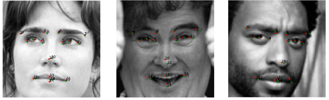
The above are some of the predictions which match closely with the ground truth data.

Now, a few bad predictions on the validation data.

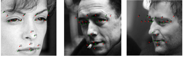
The model is predicting the keypoints around the eyes badly. In some cases, the mouth keypoints are not so good as well.

The following figure shows a few of the keypoints prediction results from the test data.

Although we do not have the ground truth data for the test images, still most of the results look pretty good here.

A Few Takeaways, Advantages, and Disadvantages

This completes our implementation of simple facial keypoint detection using TensorFlow and Keras in this tutorial.

One of the advantages of the current approach is that our model is very simple with less than 2 million parameters. This means that it will be pretty fast even during video inference.

But there are a few disadvantages as well. For example, our model has been trained on grayscale images and will not work on RGB images. To carry out image and video inference on RGB images, we will need to train another model on RGB images. Or convert the RGB images to grayscale which is not very convenient.

For further experiments, we can try out the following things:

• We can try building a larger model and see how it performs.
• Maybe even train on larger images by resizing them.
• We can also try and augment the images. But we need to be careful, as we will have to take care of the keypoint transforms in that case also.

If you try out any of the above, do let others know about your results in the comment section.

Summary and Conclusion

We covered a very simple training pipeline for facial keypoint detection using TensorFlow and Keras here. We analyzed the training and inference results and discussed some of the key advantages and disadvantages. I hope that this tutorial was helpful to you.

If you have any doubts, thoughts, or suggestions, please leave them in the comment section. I will surely address them.

You can contact me using the Contact section. You can also find me on LinkedIn, and Twitter.