An Introduction to PyTorch Visualization Utilities

Training of neural networks models is pretty important in deep learning. A good model is literally the difference between good AI software and bad AI software. But there is another important aspect of deep learning based computer vision programs and training pipelines. That is proper visualization of the outputs. This is even more important when we are dealing with outputs of object detection, semantic segmentation, instance segmentation, and keypoint detection neural network models. Annotating the output images properly can give a very good insight and can prevent the user from asking unnecessary questions. For annotations, post-processing of images or frames using OpenCV is a common option. But did you know we can do all those things using native PyTorch as well? And perhaps even better. This tutorial is going to be a simple introduction to PyTorch visualization utilities.

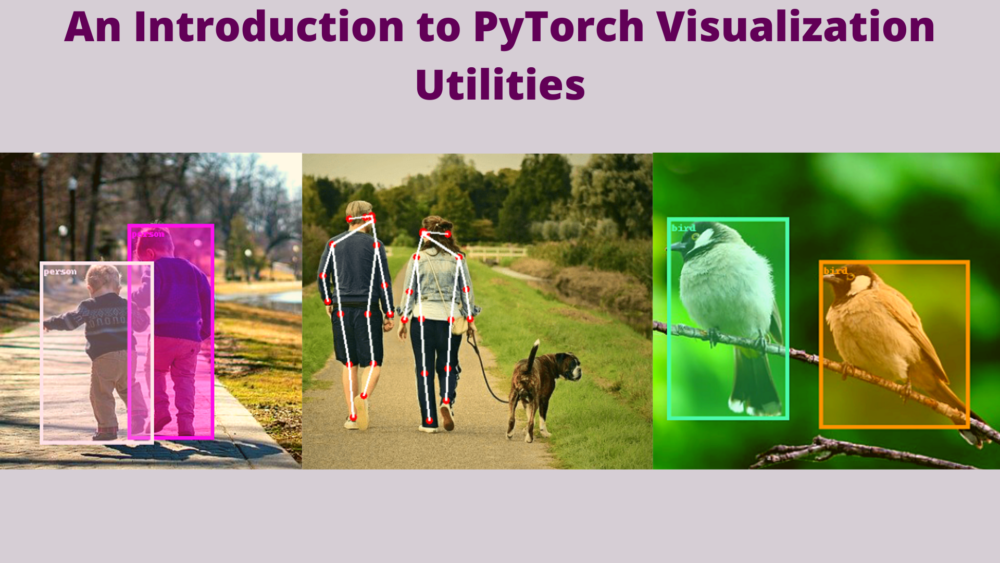
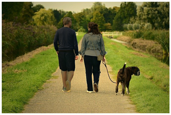
The above object detection bounding boxes were annotated using PyTorch visualization utilities. If you would like to know how it was done, keep reading this introduction to PyTorch visualization utilities post.

Topics that we are going to cover in this post.

• We will start with why we may consider using PyTorch visualization utilities rather than other libraries like OpenCV.
• Then we will slowly move on to using the PyTorch visualization utilities on different tasks like:
  • Drawing bounding boxes around objects.
  • Segmenting objects in semantic segmentation.
  • Drawing bounding boxes and segmenting objects in instance segmentation.
  • Drawing keypoints on persons for keypoint detection.

Let’s jump into the details of the post now.

Why Do We Need an Introduction to PyTorch Visualization Utilities?

Note that this tutorial has been adapted from this PyTorch tutorial. We will cover the concepts a bit more in-depth here while trying to answer questions like “why do we need to do this in a particular way?”

It is very common for deep learning practitioners to use OpenCV for annotations in deep learning project outputs. We may use it for drawing bounding boxes around objects, overlaying segmentation maps, or even drawing keypoints. Although the process is easy and straightforward, it leads us to move away from the native data format that we may already be using in the PyTorch code.

Let’s answer why do we need to know about PyTorch visualization utilities using three simple points.

• First of all, we will not be dependent on any other libraries for visualization and annotations.
• Secondly, everything will happen in a streamlined manner in the same PyTorch pipeline.
• Lastly, which is not exactly a major concern, as PyTorch visualization utilities use PIL for image annotations, they will be clearer and sharper. A point nonetheless.

Although the above points may not be very major motives to right away switch to PyTorch visualization utilities. Still, there is no harm in learning a new tool of a deep learning library.

Directory Structure

Let’s take a look at the directory structure for this tutorial.

├── input
│   ├── image_1.jpg
│   ├── image_2.jpg
│   └── image_3.jpg
└── visualization_utilities.ipynb

Here, we have one input directory containing the images that we will use for annotations and visualizations. And, there is one Jupyter Notebook, that is, visualization_utilities.ipynb containing all the code.

We will keep the code very simple and straightforward here. As understanding the concepts is the main objective here, we will focus a bit less on the modularity of the code.

PyTorch Version

All the code in this tutorial uses torch 1.11.0 and torchvision 0.12.0. If you need to install/upgrade your PyTorch version, you can visit the official website and install it as per your requirements.

Code for PyTorch Visualization Utilities

In this section, we will start with the coding part for the post. Note that all the code is available in the Jupyter notebook that you can download in this post.

Let’s start with the importing of the modules that we need here. The following are a few of the imports that we need right away. We will import the remaining modules and libraries in the specific sections where we need them.

import torch
import numpy as np
import matplotlib.pyplot as plt
import torchvision.transforms.functional as F
import os

# To make grid of images.
from torchvision.utils import make_grid
from torchvision.io import read_image
from PIL import Image

Let’s go over some of the important imports.

• make_grid: This is a PyTorch function that accepts a list of tensor images and makes a grid out of them. This is a bit similar to Matplotlib’s subplot function. But here, we can provide the tensors directly to the make_grid function without any further conversion.
• read_image: This torchvision function reads an image directly in tensor format where the channel of the image is the first dimension. So, the image has a shape [C, H, W] by default.

Also, we will need Image module from PIL to read images when we don’t need them directly in the tensor format.

Visualizing a Grid of Images

We can visualize multiple images in a grid after converting them to the appropriate format using the make_grid function.

Before we can do that, the following code cell defines the three image paths that are inside the input directory and reads them.

image_1_path = os.path.join('input', 'image_1.jpg')
image_2_path = os.path.join('input', 'image_2.jpg')
image_3_path = os.path.join('input', 'image_3.jpg')

image_1 = read_image(image_1_path)
image_2 = read_image(image_2_path)
image_3 = read_image(image_3_path)

We are using the read_image function from torchvision.

The make_grid expects every image to be of the same shape. So, let’s resize them to 450×450 dimensions.

image_1 = F.resize(image_1, (450, 450))
image_2 = F.resize(image_2, (450, 450))
image_3 = F.resize(image_3, (450, 450))

We are using the resize function from the torchvision.transforms.functional module.

The next code block does three things:

• Prepares the grid of images.
• Defines a show function for visualization.
• And shows the grid of images.

grid = make_grid([image_1, image_2, image_3])

def show(image):
    plt.figure(figsize=(12, 9))
    plt.imshow(np.transpose(image, [1, 2, 0]))
    plt.axis('off')

show(grid)

The make_grid function accepts the image tensors as a list. And the show function is a general visualization function that we will use throughout the post for visualizing different results.

The above figure shows the grid result. You might be able to realize how easily we were able to do this without any looping over the images. This is one of the benefits of using the PyTorch visualization utilities.

Drawing and Visualizing Bounding Boxes

Next, let’s move over to drawing and visualizing bounding boxes using the PyTorch visualization utilities.

First, we will do it manually, then check out how to do it by drawing the bounding boxes that are detected by an object detection model.

The first thing that we need here is to import the draw_bounding_boxes function.

# For drawing bounding boxes.
from torchvision.utils import draw_bounding_boxes

The next step is defining a tensor containing lists of bounding boxes, defining a list containing color names, and drawing the bounding boxes on the image.

boxes = torch.tensor([
    [135, 50, 210, 365], 
    [210, 59, 280, 370],
    [300, 240, 375, 380]
])
colors = ['red', 'red', 'green']
result = draw_bounding_boxes(
    image=image_1, 
    boxes=boxes, 
    colors=colors, 
    width=3
)
show(result)

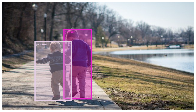
In the above code, boxes is a tensor containing lists of bounding box coordinates in [x_min, y_min, x_max, y_max] format. The colors list contains the names of colors, one for each bounding box, in the form of a string. Then we use the draw_bounding_boxes function while passing the appropriate values to the arguments. They are quite self-explanatory. Finally, we visualize the result.

Here, we draw the bounding boxes for the humans in red color and one for the dog in green. As you may observe, we provided the colors as string names. But it may not be always appropriate to do so. Instead, we can also give them as tuple values in RGB format which opens up a lot more possibilities. Let’s replicate the above colors in RGB tuple values.

colors = [(255, 0, 0), (255, 0, 0), (0, 255, 0)]
result = draw_bounding_boxes(
    image_1, boxes=boxes, 
    colors=colors, width=3
)
show(result)

The above code should essentially give the same result. The shade of the green color may be a bit different because of how the function perceives different methods for color. But it should not be a very drastic change.

Plotting Bounding Boxes from Torchvision Detection Models

It is now time to move to the interesting parts. We know that in deep learning, we often annotate the outputs of an object detection model. Let’s do that here as well using the above function.

We start with importing an object detection model and the transforms module.

from torchvision.models.detection import fasterrcnn_resnet50_fpn
from torchvision import transforms as transforms

We will use the Faster RCNN ResNet50 FPN pretrained model for object detection here.

Next, let’s define the MS COCO class names.

COCO_INSTANCE_CATEGORY_NAMES = [
    '__background__', 'person', 'bicycle', 'car', 'motorcycle', 'airplane', 'bus',
    'train', 'truck', 'boat', 'traffic light', 'fire hydrant', 'N/A', 'stop sign',
    'parking meter', 'bench', 'bird', 'cat', 'dog', 'horse', 'sheep', 'cow',
    'elephant', 'bear', 'zebra', 'giraffe', 'N/A', 'backpack', 'umbrella', 'N/A', 'N/A',
    'handbag', 'tie', 'suitcase', 'frisbee', 'skis', 'snowboard', 'sports ball',
    'kite', 'baseball bat', 'baseball glove', 'skateboard', 'surfboard', 'tennis racket',
    'bottle', 'N/A', 'wine glass', 'cup', 'fork', 'knife', 'spoon', 'bowl',
    'banana', 'apple', 'sandwich', 'orange', 'broccoli', 'carrot', 'hot dog', 'pizza',
    'donut', 'cake', 'chair', 'couch', 'potted plant', 'bed', 'N/A', 'dining table',
    'N/A', 'N/A', 'toilet', 'N/A', 'tv', 'laptop', 'mouse', 'remote', 'keyboard', 'cell phone',
    'microwave', 'oven', 'toaster', 'sink', 'refrigerator', 'N/A', 'book',
    'clock', 'vase', 'scissors', 'teddy bear', 'hair drier', 'toothbrush'
]

Now, the detection threshold and the transforms for tensor conversion.

detection_threshold = 0.8

transform = transforms.Compose([
        transforms.ToTensor(),
])

Following that, we have a function that reads an image and returns two different tensor formats for the same. We will check out the code first, then go over the explanation.

def read_transform_return(image_path):
    image = Image.open(image_path)
    image = np.array(image)
    image_transposed = np.transpose(image, [2, 0, 1])
    # Convert to uint8 tensor.
    int_input = torch.tensor(image_transposed)
    # Convert to float32 tensor.
    tensor_input = transform(image)
    tensor_input = torch.unsqueeze(tensor_input, 0)
    return int_input, tensor_input

The read_transform_return function reads the image using PIL’s Image module from the image_path that we provide as an argument. After converting the image to a NumPy array, we transpose the dimensions to bring the channel dimension to the front (as per PyTorch format). Then we convert it into both uint8 tensor format using torch.tensor, and float32 tensor format using the transform defined above. We need two different formats because all the PyTorch visualization utilities accept only uint8 tensors for annotations, and for forward propagating through the model, we need float32 tensors. In the end, the function returns the int_input and tensor_input, in uint8 format and float32 format respectively.

The above function is important because we will be using it whenever we need images for annotations and predictions.

The following code block reads the image using the above function, initializes the model, and forward propagates the appropriate tensor through the model.

int_input, tensor_input = read_transform_return(image_1_path)
model = fasterrcnn_resnet50_fpn(pretrained=True, min_size=800)
model.eval()

outputs = model(tensor_input)

Next, let’s filter out the output bounding boxes and classes according to detection_threshold.

pred_scores = outputs[0]['scores'].detach().cpu().numpy()
pred_classes = [COCO_INSTANCE_CATEGORY_NAMES[i] for i in outputs[0]['labels'].cpu().numpy()]
pred_bboxes = outputs[0]['boxes'].detach().cpu().numpy()
boxes = pred_bboxes[pred_scores >= detection_threshold].astype(np.int32)
pred_classes = pred_classes[:len(boxes)]

Now, we define tuples of RGB colors as per the number of bounding boxes left after thresholding.

colors=np.random.randint(0, 255, size=(len(boxes), 3))
colors = [tuple(color) for color in colors]

Drawing Unfilled Bounding Boxes with Appropriate Labels

Now, passing all the required arguments though draw_bounding_boxes and showing the results.

result_with_boxes = draw_bounding_boxes(
    image=int_input, 
    boxes=torch.tensor(boxes), width=4, 
    colors=colors,
    labels=pred_classes,
)

show(result_with_boxes)

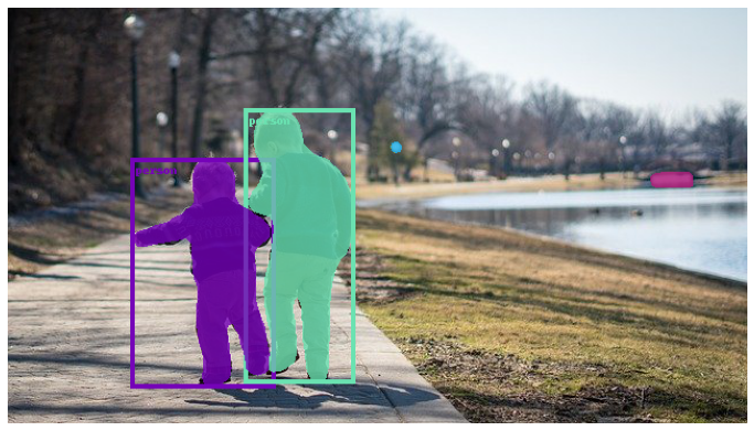
As you can see, we are passing an extra labels argument here with the pred_classes that we obtained from the outputs. This will annotate the image with appropriate classes. The following is the output.

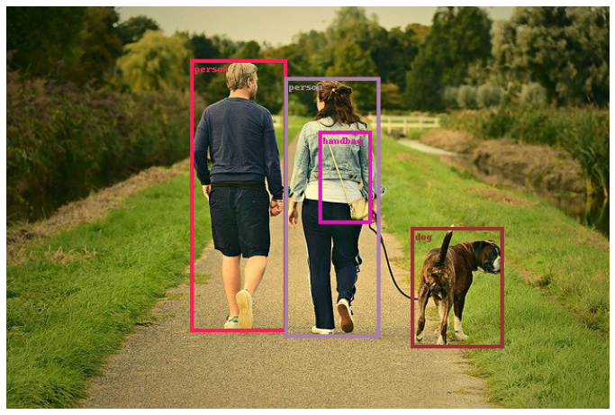
As we are choosing colors randomly, every time they will be different. Although we can set NumPy seed to avoid that.

Drawing Filled Bounding Boxes with Appropriate Labels

We can also fill the bounding boxes with colors that are the same as those of the corresponding bounding boxes. We just need to pass an extra fill argument with the value as True.

result_with_boxes = draw_bounding_boxes(
    int_input, boxes=torch.tensor(boxes), width=4, 
    colors=colors,
    labels=pred_classes,
    fill=True
)

show(result_with_boxes)

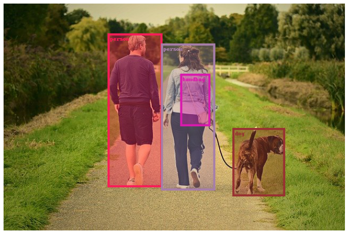
The above results with filled boxes look quite good.

Visualizing Segmentation Masks

Semantic segmentation is also an important problem domain in deep learning and computer vision. Let’s check out how to visualize and overlay segmentation masks on top of images.

We will use the FCN ResNet50 model for that which has been trained on the PASCAL VOC dataset.

from torchvision.models.segmentation import fcn_resnet50
from torchvision.utils import draw_segmentation_masks

Now, define the PASCAL VOC class names and the corresponding color map for the classes.

VOC_SEG_CLASSES = [
    '__background__', 'aeroplane', 'bicycle', 'bird', 'boat', 'bottle', 'bus',
    'car', 'cat', 'chair', 'cow', 'diningtable', 'dog', 'horse', 'motorbike',
    'person', 'pottedplant', 'sheep', 'sofa', 'train', 'tvmonitor'
]

label_color_map = [
               (0, 0, 0),  # background
               (128, 0, 0), # aeroplane
               (0, 128, 0), # bicycle
               (128, 128, 0), # bird
               (0, 0, 128), # boat
               (128, 0, 128), # bottle
               (0, 128, 128), # bus 
               (128, 128, 128), # car
               (64, 0, 0), # cat
               (192, 0, 0), # chair
               (64, 128, 0), # cow
               (192, 128, 0), # dining table
               (64, 0, 128), # dog
               (192, 0, 128), # horse
               (64, 128, 128), # motorbike
               (192, 128, 128), # person
               (0, 64, 0), # potted plant
               (128, 64, 0), # sheep
               (0, 192, 0), # sofa
               (128, 192, 0), # train
               (0, 64, 128) # tv/monitor
]

Visualizing Boolean Masks

Let’s start with visualizing a boolean mask. This means, all the segmented objects of interest with be highlighted in the same way irrespective of the class they belong to. The following code block contains the entire code for that.

int_input, tensor_input = read_transform_return(image_1_path)

model = fcn_resnet50(pretrained=True)
model.eval()
outputs = model(tensor_input)

labels = torch.argmax(outputs['out'][0].squeeze(), dim=0).detach().cpu().numpy()
boolean_mask = torch.tensor(labels, dtype=torch.bool)

seg_result = draw_segmentation_masks(
    image=int_input, 
    masks=boolean_mask,
    alpha=0.5
)

show(seg_result)

First, we obtain the respective tensors by reading the image, then carry out the prediction using the model. Then we obtain a boolean_mask by applying argmax to outputs['out'][0] which contains the segmentation mask results. We apply it across dim=0. Now anywhere in the output mask, if the value is greater than 0 (not background), that index will have the value True in boolean_mask.

Next, we use the draw_segmentation_masks function which accepts the following arguments:

• image: An uint8 tensor.
• masks: The resulting mask to overlay on the image.
• alpha: A float value indicating the transparency of the masks.

This gives us the following result.

We can see that the two persons and the dog are having darker masks and the background is clear.

Visualizing RGB Masks

But that’s not all. We can also apply colors to the output masks according to the PASCAL VOC classes.

The following code shows how to do that.

num_classes = outputs['out'].shape[1]
masks = outputs['out'][0]
class_dim = 0 # 0 as it is a single image and not a batch.
all_masks = masks.argmax(class_dim) == torch.arange(num_classes)[:, None, None]

First, we obtain the number of classes and the masks from the outputs. Then we obtain a all_masks tensor by applying argmax across dimension 0 and wherever the value is matching the class number of torch.arange(num_classes). Here, we use class_dim=0 as we have a single image only and not a batch of images.

Then we just need to pass the above obtained all_masks to the draw_segmentation_masks function.

seg_result = draw_segmentation_masks(
    int_input, 
    all_masks,
    colors=label_color_map,
    alpha=0.5
)

show(seg_result)

This time, we pass the label_color_map list of tuples as a value to the colors argument so that the function can overlay the segmentation maps with appropriate colors.

The above image shows the output with RGB masks.

Visualization for Instance Segmentation Models

Instance segmentation is another important field in deep learning and computer vision. In instance segmentation, we need to draw the bounding boxes and apply segmentation masks on each object and that too with a different color.

We have already seen above how to do both individually. Let’s try to combine them now.

We will use the Mask RCNN ResNet50 FPN model for instance segmentation.

from torchvision.models.detection import maskrcnn_resnet50_fpn

Reading the image and getting outputs.

int_input, tensor_input = read_transform_return(image_3_path)

model = maskrcnn_resnet50_fpn(pretrained=True)
model.eval()
outputs = model(tensor_input)

Now, let’s extract the bounding boxes and masks out of those predictions.

output = outputs[0]
masks = output['masks']
boxes = output['boxes']

We will apply the same thresholding formula as we did above for the bounding boxes.

detection_threshold = 0.8
pred_scores = outputs[0]['scores'].detach().cpu().numpy()
pred_classes = [COCO_INSTANCE_CATEGORY_NAMES[i] for i in outputs[0]['labels'].cpu().numpy()]
pred_bboxes = outputs[0]['boxes'].detach().cpu().numpy()
boxes = pred_bboxes[pred_scores >= detection_threshold].astype(np.int32)
pred_classes = pred_classes[:len(boxes)]

Then we define the colors for the bounding boxes and draw the bounding boxes on the tensor image.

colors = np.random.randint(0, 255, size=(len(COCO_INSTANCE_CATEGORY_NAMES), 3))
colors = [tuple(color) for color in colors]
result_with_boxes = draw_bounding_boxes(
    int_input, boxes=torch.tensor(boxes), width=4, 
    colors=colors,
    labels=pred_classes,
)

Right now, result_with_boxes contains an image where the bounding boxes are already drawn. Next, we will pass the same image as an input to the draw_segmentation_masks.

final_masks = masks > 0.5
final_masks = final_masks.squeeze(1)

seg_result = draw_segmentation_masks(
    result_with_boxes, 
    final_masks,
    colors=colors,
    alpha=0.8
)

show(seg_result)

First, we obtain the masks where the value is above 0.5 as that indicates an object. Then we remove the second dimension, giving us the shape of final_masks as [num_obects, height, width]. Finally, we apply the segmentation masks to the above image tensor and visualize the results.

The color of the segmentation maps and bounding boxes will remain the same for a particular object.

Visualizing Keypoints

Till now, in this introduction to PyTorch visualization utilities, we have covered drawing bounding boxes and segmentation maps. Now, in this final section of the tutorial, we will cover the drawing of keypoints on images.

Annotating keypoints on images using OpenCV can be complicated. We have to write our own custom loop. Here, we will observe how easy that process becomes.

We will use the Keypoint RCNN ResNet50 FPN model here.

Let’s import the model and required function.

from torchvision.models.detection import keypointrcnn_resnet50_fpn
from torchvision.utils import draw_keypoints

PyTorch provides the draw_keypoints function to draw the keypoints in the images.

Now, let’s define the keypoint body parts and connection points for drawing the keypoint skeleton later on.

COCO_KEYPOINTS = [
    "nose", "left_eye", "right_eye", "left_ear", "right_ear",
    "left_shoulder", "right_shoulder", "left_elbow", "right_elbow",
    "left_wrist", "right_wrist", "left_hip", "right_hip",
    "left_knee", "right_knee", "left_ankle", "right_ankle",
]

CONNECT_POINTS = [
    (0, 1), (0, 2), (1, 3), (2, 4), (0, 5), (0, 6), (5, 7), (6, 8),
    (7, 9), (8, 10), (5, 11), (6, 12), (11, 13), (12, 14), (13, 15), (14, 16)
]

The CONNECT_KEYPOINTS defines the index positions from COCO_KEYPOINTS which will be connected with each other. This means that nose will be connected with left_eye, then nose with right_eye and so on.

Next, read the image and pass the tensor through the model.

int_input, tensor_input = read_transform_return(image_1_path)

model = keypointrcnn_resnet50_fpn(pretrained=True)
model.eval()
outputs = model(tensor_input)

Here are the next few steps that we perform.

• We extract the keypoints and scores from the output.
• Then we filter out the keypoints which are below the detection threshold score.
• Next, we draw just the points on the image.

keypoints = outputs[0]['keypoints']
scores = outputs[0]['scores']

idx = torch.where(scores > detection_threshold)
keypoints = keypoints[idx]

keypoints_results = draw_keypoints(
    image=int_input, 
    keypoints=keypoints,
    colors=(255, 0, 0),
    radius=2
)

show(keypoints_results)

In the above block, the keypoints argument accepts the filtered out keypoints that we obtained above from the model output. The radius argument defines the radius of the keypoint circles.

Right now, we have the following output with us.

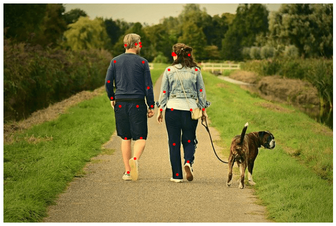
We have annotated the images with the keypoints only.

Let’s check out the code that annotates the image with the skeletal line as well.

final_kpts_result = draw_keypoints(
    image=int_input, 
    keypoints=keypoints, 
    connectivity=CONNECT_POINTS, 
    colors=(255, 0, 0), 
    radius=4, 
    width=3
)

show(final_kpts_result)

This time, we provide two more arguments:

• connectivity: This accepts the CONNECT_POINTS list which contains which body parts are connected with each other.
• width: To define the width of the skeletal lines.

The final result looks like the following.

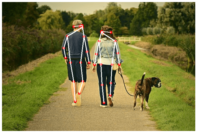
Finally, we draw the keypoints and skeletal lines also in this introduction to PyTorch visualization utilities post. As you can see, we did not use any loops and were able to draw the keypoints and the connecting skeletal lines pretty easily.

Summary and Conclusion

In this introduction to PyTorch visualization utilities tutorial, we went through several functions that PyTorch provides for easy visualization of bounding boxes, segmentation maps, and keypoints. In the next tutorial, we will check out how to integrate all these functionalities into an image and video inference pipeline. I hope that this tutorial was helpful to you.

If you have any doubts, thoughts, or suggestions, please leave them in the comment section. I will surely address them.

You can contact me using the Contact section. You can also find me on LinkedIn, and Twitter.