Basic Introduction to Class Activation Maps in Deep Learning using PyTorch

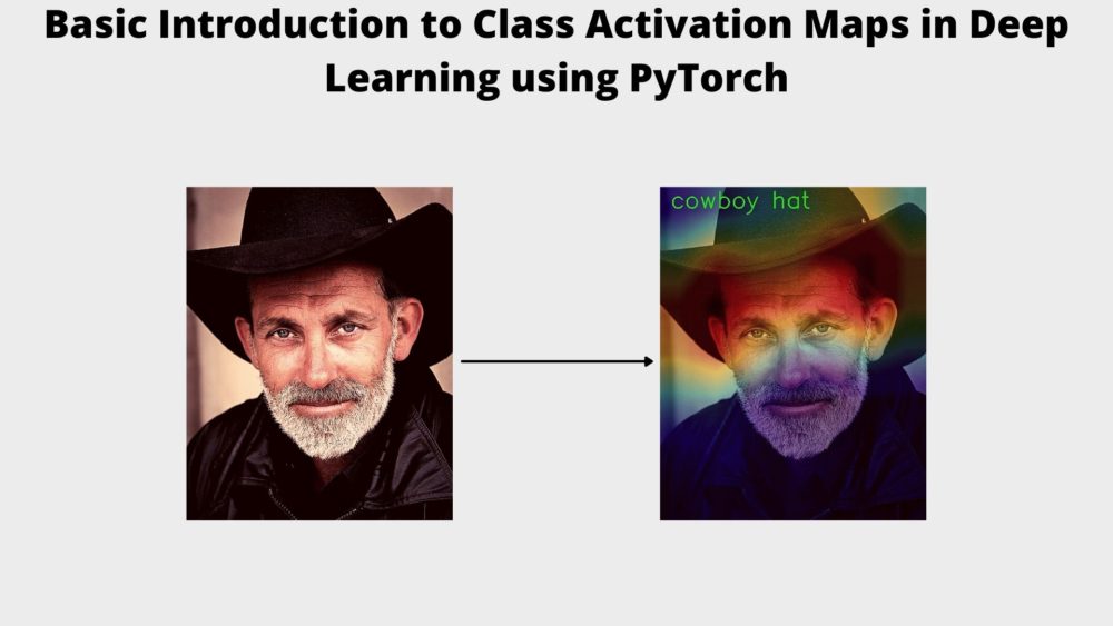
By now you must have trained a number of deep learning image classification models. That may be on a custom dataset or very classic computer vision datasets like MNIST or CIFAR10. And you must have also carried out inference using many state-of-the-art image classification models like ResNets and VGG nets. Or even newer models like EfficientNets. After all these experiments, there is one interesting question that arises. How does a deep learning model know whether it is looking at a cat or a dog or a tiger? And if it is looking at a tiger, what is it in the image that leads the model to predict it as a tiger? To answer this, we can use Class Activation Maps (CAM). In this blog post, we will be learning about Class Activation Maps in deep learning using PyTorch.

What are we going to cover in this article?

• A brief introduction to Class Activation Maps in Deep Learning.
• A very simple image classification example using PyTorch to visualize Class Activation Maps (CAM).
  • We will use a ResNet18 neural network model which has been pre-trained on the ImageNet dataset..

Note: We will not cover the theory and concepts extensively in this blog post. This is a very simple introduction to Class Activation Maps in deep learning in PyTorch with a code first approach. We will cover deep learning computer vision model interpretability in detail in future posts. These include:

• Class Activation Maps in detail along with coding in PyTorch and theory as well.
• GradCAM in detail.
• Custom training and visualizing CAM on the custom test dataset.
• We will also cover many of the papers in the field in detail.

A Brief Introduction to Class Activation Map (CAM) in Deep Learning

For many years, deep learning researcher and practitioners alike thought deep neural networks to be black box. We know what input we give to the model and we also get the output. But we were unable to justify why a neural network took a specific detection? What did an image classification model see in the image that made it predict that the image contains a dog?

Specifically, we use something called as Class Activation Map (CAM). This indicates a region in an image that a Convolutional Neural Network uses to predict the class of the image. In terms of applications, this can be seen as a heatmap that we can overlay on top of the original image to see why the CNN model predicted a specific label for an image.

Paper and Concept

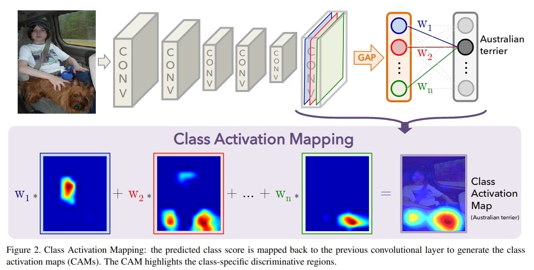
The concept of Class Activation Map was introduced by Zhou et al in the paper Learning Deep Features for Discriminative Localization. They use the term Class Activation Maps to refer to weighted activation maps generated by a CNN. These weighted activations lead to the prediction of a specific label for the image.

You can also find the sample code for the paper here.

To make our understanding more concrete, let us take a look at an example.

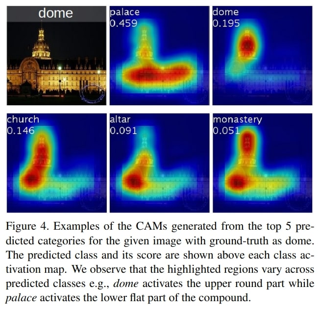
In the above image, we see at the top left corner that the ground truth is dome. The five image blocks with the CAM show the top-5 predictions with their respective CAM highlighting and which region in the image leads the CNN to predict that the image belonged to that class.

For each of the top-5 predictions, the CNN predicts a different class based on the weighted activation maps.

There are many more details, we have barely scratched the surface of such an interesting topic. What we discussed can help us in understanding a very basic coding example using PyTorch. And that is what we are going to do in this blog post. We will not dive any deeper into the paper or theory in this blog post. Instead, we will focus on visualizing Class Activation Maps in Deep Learning using PyTorch. As such, we will use a pre-trained ResNet18 (trained on the ImageNet dataset) model in this tutorial to learn about class activation maps.

The Directory Structure

The following is the directory structure that we will stick to for this mini project.

├── cam.py
├── input
│   ├── image_1.jpg
│   └── image_2.jpg
├── LOC_synset_mapping.txt
├── outputs
│   ├── CAM_image_1.jpg
│   └── CAM_image_2.jpg

• In the input folder we have a few images that we will feed into the neural network to visualize the Class Activation Maps.
• The cam.py is the only Python script that we need which will contain all the code needed to visualize the CAM after the images have passed through the neural network.
• The outputs folder will contain the Class Activation Map images where the class activation heatmap will be overlayed on top of the original input image.
• Finally, we have a LOC_synset_mapping.txt which contains all the ImageNet labels. We will use this text file to map the neural network’s predictions to the labels.

You are free to use your own images as well.

PyTorch Version

Although you should be fine using any of the PyTorch 1.6+ versions. Still, to avoid any unseen errors, you can use the same version as this tutorial, which is PyTorch 1.8.0. If you wish to download the latest version of PyTorch, you can do it from the official site.

Class Activation Maps in Deep Learning using PyTorch

From this section onward, we will focus on the coding part of the blog post. We will use two images for the class activation map visualization using PyTorch.

The following are the images that we have in the input folder.

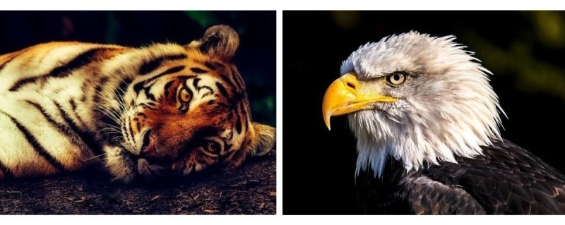
One image is of a tiger (ground truth is tiger) and the other image is of an eagle (ground truth is bald eagle). It will be interesting to see whether the ResNet18 model can predict the classes correctly or not. And what parts of the images the model focuses on for making the predictions.

The code that we will cover here is inspired from this code which is a PyTorch example of CAM. I have changed the code as required for this blog post.

All the code that we will write will go into the cam.py Python script.

Let us start with the import statements.

import numpy as np
import cv2
import argparse

from torchvision import models, transforms
from torch.nn import functional as F
from torch import topk

• We will need the transforms and models from torchvision to apply transforms to the image and load the ResNet18 model.
• We are importing topk from torch that will help us to get the top k probabilities from the model outputs. For example, if we want to get the top 5 probabilities, we can easily get using using topk(probs, 5).

Construct the Argument Parser

The next block of code constructs the argument parser to parse the command line arguments.

# construct the argument parser
parser = argparse.ArgumentParser()
parser.add_argument('-i', '--input', help='path to input image', 
                    default='input/image_1.jpg')
args = vars(parser.parse_args())

The --input flag will accept the path to the input image that we will provide while executing the script.

Next, we will cover a few functions that will help us along the way for the class activation map visualization.

Function to Generate the Class Activation Map

We will write a function to generate the class activation map. This function has been taken from this PyTorch code.

# https://github.com/zhoubolei/CAM/blob/master/pytorch_CAM.py
def returnCAM(feature_conv, weight_softmax, class_idx):
    # generate the class activation maps upsample to 256x256
    size_upsample = (256, 256)
    bz, nc, h, w = feature_conv.shape
    output_cam = []
    for idx in class_idx:
        cam = weight_softmax[idx].dot(feature_conv.reshape((nc, h*w)))
        cam = cam.reshape(h, w)
        cam = cam - np.min(cam)
        cam_img = cam / np.max(cam)
        cam_img = np.uint8(255 * cam_img)
        output_cam.append(cv2.resize(cam_img, size_upsample))
    return output_cam

Basically, the returnCAM() function generates the class activation maps based on the convolutional features of the ResNet18 model, the weighted softmax parameters, and the class indices. The for loop from line 19 will run as many times as the number of class indices present in class_idx. This number will be the same as the number of top k probabilities we choose.

Finally, it returns the output_cam list which contains the class activation maps.

Function to Overlay and Show the Class Activation Map on the Original Image

We will overlay the class activation map on top of the original image for proper visualization. Before that we need to generate a type of heatmap from the class activations. The following show_cam() function helps in achieving that.

def show_cam(CAMs, width, height, orig_image, class_idx, all_classes, save_name):
    for i, cam in enumerate(CAMs):
        heatmap = cv2.applyColorMap(cv2.resize(cam,(width, height)), cv2.COLORMAP_JET)
        result = heatmap * 0.3 + orig_image * 0.5
        # put class label text on the result
        cv2.putText(result, all_classes[class_idx[i]], (20, 40), 
                    cv2.FONT_HERSHEY_SIMPLEX, 1.5, (0, 255, 0), 2)
        cv2.imshow('CAM', result/255.)
        cv2.waitKey(0)
        cv2.imwrite(f"outputs/CAM_{save_name}.jpg", result)

Let us go over the parameters that the show_cam() function accepts:

• CAMs is the class activation map list that we got from the returnCAM() function. That is, the output_cam list.
• The width and height are the original width and height of the image that we will read.
• The orig_image is the original NumPy array image without any normalizations or transformations.
• class_idx contains the class indices for the top k softmax probabilities.
• all_classes is a list containing the ImageNet labels.
• Finally, the save_name is a string containing the name using which the resulting image will be saved to disk.

First, we generate a heatmap using the activation maps at line 29. Then we obtain the resulting image by combining the heatmap and original image at line 30. At line 32, we put the class label text on the resulting image. Then we show the image on the screen and save it to disk.

Function to Load the Image Class Labels

This is going to be a very simple function that will load the class labels from the ImageNet dataset. If you have downloaded the source code by now, then the LOC_synset_mapping.txt file is already present in the project folder. Else you can also download the file from this Kaggle link.

The following is the function to load the class labels in a list.

def load_synset_classes(file_path):
    # load the synset text file for labels
    all_classes = []
    with open(file_path, 'r') as f:
        all_lines = f.readlines()
        labels = [line.split('\n') for line in all_lines]
        for label_list in labels:
            current_class = [name.split(',') for name in label_list][0][0][10:]
            all_classes.append(current_class)
    return all_classes

# get all the classes in a list
all_classes = load_synset_classes('LOC_synset_mapping.txt')

At line 49, we are calling the load_synset_classes() function by passing the class file path as the argument. Printing all_classes will give the following result now.

['tench', 'goldfish', 'great white shark', 'tiger shark', 'hammerhead', 
'electric ray', 'stingray', 'cock', 'hen', 'ostrich'
... 'gyromitra', 'stinkhorn', 'earthstar', 'hen-of-the-woods', 
'bolete', 'ear', 'toilet tissue']

So, each element in the list will refer to one class label from the ImageNet dataset.

Read and Prepare the Image

The next step is to read the image from disk and prepare it to pass it through the ResNet18 model.

# read and visualize the image
image = cv2.imread(args['input'])
orig_image = image.copy()
image = cv2.cvtColor(image, cv2.COLOR_BGR2RGB)
height, width, _ = image.shape

We are simply reading the image from the disk and then keeping a copy of the original image. Then we are converting the color format from BGR to RGB for the image that we will feed into the deep learning model at line 53. At line 54 we are extracting the height and width of the image for later use.

Load the Prepare the ResNet18 Model

The next step is to load and prepare the deep learning model. And in our case, it is a ResNet18 model.

It is important to note here that we only need the convolutional layers of the ResNet18 model and not the final classification layers. For the ResNet18 model, it is till layer4. This means we only need the convolutional feature outputs and not the actual classification predictions from the model.

The following block shows the code for that.

# load the model
model = models.resnet18(pretrained=True).eval()
# hook the feature extractor
# https://github.com/zhoubolei/CAM/blob/master/pytorch_CAM.py
features_blobs = []
def hook_feature(module, input, output):
    features_blobs.append(output.data.cpu().numpy())
model._modules.get('layer4').register_forward_hook(hook_feature)
# get the softmax weight
params = list(model.parameters())
weight_softmax = np.squeeze(params[-2].data.numpy())

• At line 56, we are loading the pre-trained ResNet18 model and switching it to evaluation mode.
• At line 60, we are defining a small function that hooks the feature extractor of the ResNet18 model. This allows us to get the model features till layer4 only. We can see that at line 62, we are extracting the features till layer4 using get() and passing the hook_feature() function to register_forward_hook().
• Line 64 extracts the model’s parameters and line 65 gets the softmax weights from the model.

You can also find the above code snippet here.

Define the Image Transforms and Normalization

Before we can feed the image to the ResNet18 neural network, we need to apply a few transforms to the image.

# define the transforms, resize => tensor => normalize
transforms = transforms.Compose(
    [transforms.ToPILImage(),
     transforms.Resize((224, 224)),
     transforms.ToTensor(),
     transforms.Normalize(
        mean=[0.485, 0.456, 0.406],
        std=[0.229, 0.224, 0.225]
    )
    ])

We will be reading the image using OpenCV. So, we are first converting the image to a PILImage() format, resizing it to 224 x 224, and converting it to a tensor. Also, because the ResNet18 model has been trained on the ImageNet dataset, we are applying the ImageNet normalization stats to the tensors.

Apply the Transforms and Forward Pass Through the Network

Now, we can apply the above transforms to the image and forward pass the data through the neural network.

# apply the image transforms
image_tensor = transforms(image)
# add batch dimension
image_tensor = image_tensor.unsqueeze(0)
# forward pass through model
outputs = model(image_tensor)
# get the softmax probabilities
probs = F.softmax(outputs).data.squeeze()
# get the class indices of top k probabilities
class_idx = topk(probs, 1)[1].int()

After applying the transforms, we are adding one extra batch dimension to the image tensor to make it of shape [1, 3, 224, 224]. This is what normally any PyTorch image model expects. We are feeding the image tensor to the neural network at line 81. Then we are applying the softmax function to get the softmax probabilities from the outputs at line 83. At line 85, we are getting the class index for the top 1 probability from all the softmax probabilities.

Generate the Class Activation Maps and Visualize the Outputs

The final few steps are:

• Generate the Class Activation Maps by calling the returnCAM() function.
• Visualize the CAM results by calling the show_cam() function.

# generate class activation mapping for the top1 prediction
CAMs = returnCAM(features_blobs[0], weight_softmax, class_idx)
# file name to save the resulting CAM image with
save_name = f"{args['input'].split('/')[-1].split('.')[0]}"
# show and save the results
show_cam(CAMs, width, height, orig_image, class_idx, all_classes, save_name)

This completes all the coding required for visualizing class activation maps in deep learning using PyTorch.

Execute cam.py and Analyze the Results

Now, we are all set to execute the cam.py script. Go into the project directory and type the following command in your terminal.

python cam.py --input input/image_1.jpg

Executing the above command should give the following output.

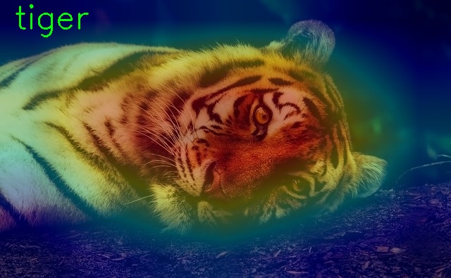
We can see that the ResNet18 model has correctly predicted the image is that of a tiger. But along with that, we can also see the heatmap on the image that shows which part in the image convinced the model to conclude that it is looking at a tiger. And rightly so, it is mostly because of the face and partly because of the striped fur as well. Looks like it is also giving us good insights into the prediction process of the model.

Let us see the results with the second image that we have.

python cam.py --input input/image_2.jpg

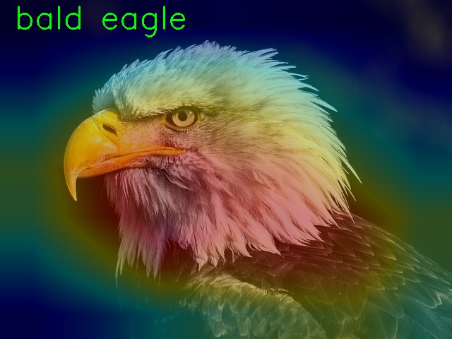
This time the head and beak of the eagle are the features which are leading the ResNet18 model to think that it is looking at a bald eagle. Pretty good actually. And pretty accurate as well.

Summary and Conclusion

In this article, we went over a very short introduction of Class Activation Maps in Deep Learning using PyTorch. Although we did not dive into the details of the topic, rather we took a code-first approach to learn about the topic and gain some initial knowledge. We will be diving into the topic in much more depth in future posts. I hope that this was helpful for you.

If you have any doubts, thoughts, or suggestions, then please leave them in the comment section. I will be happy to address them.

You can contact me using the Contact section. You can also find me on LinkedIn, and Twitter.