
Deep learning is becoming useful not only in the industrial space but also in the environmental space. Detecting animals and birds in the wild is also becoming common. Recognition, detection, and tracking of various wildlife can help speed up the study and conservation of animals. To get started with this, in this article we will carry out image classification on the Caltech UCSD Birds 200 Dataset.
We will use a pretty diverse and challenging dataset for this project. This article can help anyone who aims one of the following:
- To start using deep learning on real-life environmental use cases.
- Using deep learning to recognize different bird species in the wild.
The above list is not exhaustive. Once we have trained an image recognition model for bird species classification, we can think of various use cases.
Before we move any further, let’s take a look at all the points that we will cover in this article:
- We will start by discussing the dataset that we will use in this article.
- Next, we will move on to discuss the practical approach to training the model. This includes:
- The dataset preparation code.
- The deep learning model.
- Preparing the utility scripts.
- After we have a preliminary model trained on the dataset, we will use it for inference. This will give us a proper idea of how the model performs in the wild.
- Finally, we will also visualize classification maps generated by the model when carrying out inference.
This article will be really interesting. I hope you learn something new.
The Caltech UCSD Birds 200 Dataset
The Caltech UCSD Birds 200 is a pretty diverse and challenging dataset for bird species classification. We will use the extended version of the dataset that was updated in 2011.
This dataset contains images of 200 different species of birds. A total of 11788 images are present in the dataset. The distribution of images per class is not the same. It can vary somewhere between 40 to 60 images per class.
Not only image classification, but the dataset also supports annotations for bird body parts and bird detection also. You may find more information in the CUB-200-2011 technical report.
For our purpose, we will only focus on the classification part of the Caltech UCSD Birds 200 dataset. We will use the 200 Bird Species dataset from Kaggle for easier accessibility.
- Kaggle 200 Bird Species dataset.
Here, are a few images from the dataset along with their class names.
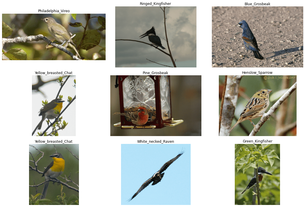
As you can see, the dataset is pretty diverse. It contains images of even the same species in varied conditions and environments. Also, it is a pretty challenging dataset. Even reaching 90% validation accuracy is a challenging task, as we will see later on.
If you download the dataset from the above link and extract it, you will find the following structure.
CUB_200_2011
├── attributes
│   ├── certainties.txt
│   ├── class_attribute_labels_continuous.txt
│   └── image_attribute_labels.txt
├── images
│   ├── 001.Black_footed_Albatross
│   ├── 002.Laysan_Albatross
│   ...
│   └── 200.Common_Yellowthroat
├── parts
│   ├── part_click_locs.txt
│   ├── part_locs.txt
│   └── parts.txt
├── bounding_boxes.txt
├── classes.txt
├── image_class_labels.txt
├── images.txt
├── README
└── train_test_split.txt
We can see various folders and files. But we are only interested in the images folder which contains the images inside the subfolders. These subfolders contain the class name prefixed with the class number. For example, 001.Black_footed_Albatross.
Although the dataset comes with train/test distribution information in the train_test_split.txt, we will use our own split during training.
For now, you may go ahead and download the dataset.
The Project Directory Structure
Let’s take a look at the Caltech UCSD Birds Classification project directory structure.
.
├── input
│   ├── CUB_200_2011
│   │   ├── attributes
│   │   ├── images
│   │   ├── parts
│   │   ├── bounding_boxes.txt
│   │   ├── classes.txt
│   │   ├── image_class_labels.txt
│   │   ├── images.txt
│   │   ├── README
│   │   └── train_test_split.txt
│   └── inference_data
│       ├── laysan_albatross.jpg
│       ├── purple_finch.jpg
│       ├── red_winged_blackbird.jpg
│       └── shiny_cowbird.jpg
├── notebooks
│   └── visualize.ipynb
├── outputs
│   ├── accuracy.png
│   ├── best_model.pth
│   ├── loss.png
│   └── model.pth
└── src
    ├── cam.py
    ├── class_names.py
    ├── datasets.py
    ├── inference.py
    ├── model.py
    ├── train.py
    └── utils.py

11 directories, 34 files
- The dataset images reside in the
input/CUB_200_2011/imagesdirectory in their respective class folder as we saw in the previous section. - We have a few inference images inside the
input/inference_datadirectory. Later on, we will use these images for inference and visualizing class activation maps. - The
notebooksdirectory contains a Jupyter Notebook to visualize the dataset and augmented images. - All the training and validation results will be stored in the
outputsdirectory. - And all the Python code files reside in the
srcdirectory. We will discuss the necessary coding details in the following section.
You can download the zip file that accompanies this article. That will give you access to the inference data, the Python files, and the Jupyter Notebook. In case you need to train the model yourself, you just need to download the dataset and arrange it in the above structure.
PyTorch Version
The whole project was developed using TORCH 1.12.0 and TORCHVISION 0.13.0. Higher versions will also work.
In case you need to install/upgrade PyTorch, do visit the official page.
Caltech UCSD Birds Classification
Starting from this section, we will discuss all the practical aspects of the post. But we will not go into the coding details. The codebase is not huge, but quite large. There are seven Python files and discussing them will be impractical for a blog post.
Instead, we will go into the details of implementation, which include:
- Which deep learning model do we use and why?
- What are the data augmentation techniques that we apply to the training set?
- How is the training script structured?
- And an overall of which things worked and which did not work?
If you wish to run the training experiments yourself, you can easily download the zip file that gives you access to all the code and inference data.
All in all will treat this as a project and we will cover more such projects/topics in the future. Let’s dive into it.
Download Code
The Utility Script
We have a utils.py file in the src directory. Without going into too many details, the script takes care of the following points:
- It contains a Python class to save the best model according to the validation loss.
- It also contains a Python function for saving the final model.
- And it has a simple function to save the loss and accuracy graphs.
Preparing the Caltech UCSD Birds Classification Dataset
The dataset comes with a train_test_split.txt file indicating which file belongs to the training set and which one to the test set.
However, we prepare the training and validation sets on the fly using the ImageFolder class. As the training script uses a seed value for reproducibility, this should not be an issue.
Now, getting into the data augmentation part. You may have observed that almost all the images have the bird at the center of the frame. This means that we can easily crop the image to some extent.
Further, although the dataset is quite large with 200 classes and more than 11000 images. Each class does not contain that many images. There are 60 images for each class (at maximum). So, this means that we need to apply a pretty good amount of augmentations as well.
But again, the colors of the birds are a very good determinant of their class. So, we cannot apply any pixel-wise color augmentations, or else the model will not get to see the actual features.
Finally, we choose the following data pipeline:
- Resize the images to 256×256 resolution.
- Apply center cropping and make them 224×224 pixels.
Then, apply the following augmentations:
RandomHorizontalFlipwith 0.5 probability.RandomVerticalFlipwith 0.5 probability.RandomRotationto rotate the images in a 35 degrees range.
The final images after the entire data pipeline look like the following:
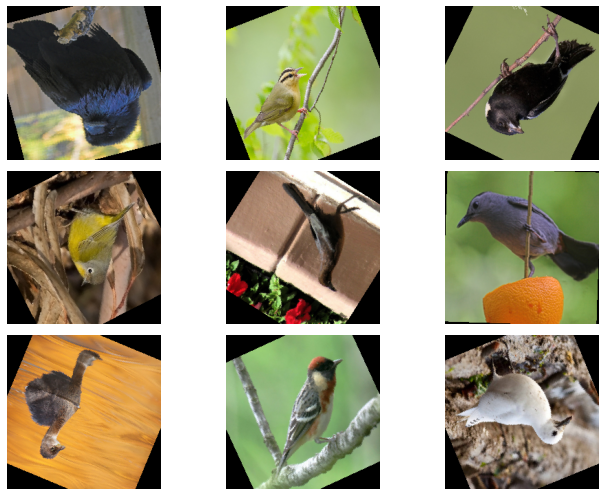
As you can see, the images look pretty varied now. This should make up for the less number of images per class.
The Deep Learning Model
We will be fine-tuning the EfficientNetB1 model on the Caltech UCSD Birds Classification dataset. The train.py script contains all the training code.
There are a few details that we need to go through before we can start the training.
- We will fine-tune the entire model. From experiments, I found that fine-tuning all the layers gave the best results.
- We will train for 45 epochs in total.
- The initial learning rate is 0.01 using the SGD optimizer. We use StepLR as the learning rate scheduler to reduce the learning rate by a factor of 10 at epoch numbers 15 and 30. Otherwise, the model seemed to overfit.
- Further, the batch size that we use here is 64. You can reduce the batch size in case you run Out Of Memory during training.
All the training experiments were done on a machine with 10 GB RTX 3080 GPU, i7 10th generation CPU, and 32 GB of RAM.
To start the training, execute the following command in the terminal within the src directory.
python train.py --epochs 45 --batch-size 64 -lr 0.01 --fine-tune
Following is the truncated output from the terminal.
[INFO]: Number of training images: 10020
[INFO]: Number of validation images: 1768
[INFO]: Classes: ['001.Black_footed_Albatross', '002.Laysan_Albatross', ... '200.Common_Yellowthroat']
Computation device: cuda
Learning rate: 0.01
Epochs to train for: 45

[INFO]: Fine-tuning all layers...
.
.
.
6,769,384 total parameters.
6,769,384 training parameters.
Adjusting learning rate of group 0 to 1.0000e-02.
[INFO]: Epoch 1 of 45
Training
100%|█████████████████████████████████████████| 157/157 [01:19<00:00,  1.98it/s]
Validation
100%|███████████████████████████████████████████| 28/28 [00:12<00:00,  2.27it/s]
Training loss: 5.081, training acc: 6.677
Validation loss: 4.394, validation acc: 24.321

Best validation loss: 4.394204889025007

Saving best model for epoch: 1

Adjusting learning rate of group 0 to 1.0000e-02.
--------------------------------------------------
.
.
.
[INFO]: Epoch 44 of 45
Training
100%|█████████████████████████████████████████| 157/157 [01:15<00:00,  2.07it/s]
Validation
100%|███████████████████████████████████████████| 28/28 [00:10<00:00,  2.56it/s]
Training loss: 0.134, training acc: 97.076
Validation loss: 0.699, validation acc: 81.505
Adjusting learning rate of group 0 to 1.0000e-04.
--------------------------------------------------
[INFO]: Epoch 45 of 45
Training
100%|█████████████████████████████████████████| 157/157 [01:14<00:00,  2.10it/s]
Validation
100%|███████████████████████████████████████████| 28/28 [00:11<00:00,  2.35it/s]
Training loss: 0.129, training acc: 97.415
Validation loss: 0.700, validation acc: 81.618
Adjusting learning rate of group 0 to 1.0000e-04.
--------------------------------------------------
TRAINING COMPLETE
The best model was saved on epoch 34. We will use this model while running inference on unseen images and visualizing class activation maps.
For the best epoch, the validation loss was 0.690 and the validation accuracy was 81.22%. This is not bad but perhaps a bigger model will perform much better on this dataset.
Let’s take a look at the accuracy and loss graphs to get more insights.
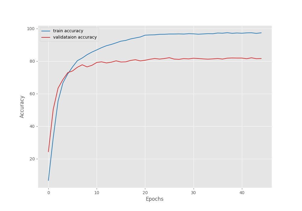
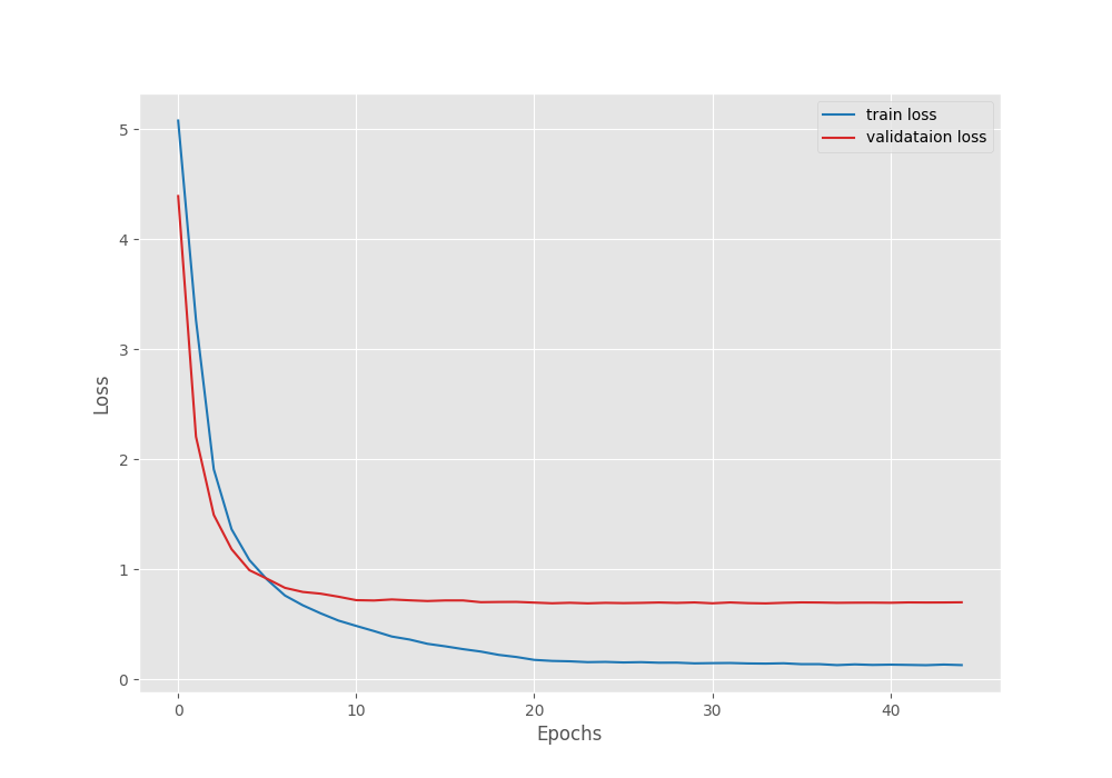
As we can see, both, the validation accuracy and validation loss curve flatten out during the final epochs. It may seem that reducing the learning rate a bit later may help. But reducing the learning rate at 20 and 40 epochs led to overfitting.
Inference and Visualizing Class Activation Maps on Images
We have the best model with us which has been trained on the Caltech UCSD Birds Classification. The inference.py script contains the code to run inference using the best model from a directory with images.
Let’s run the script and check out the results on 8 unseen images. These images have been taken from the internet and are not part of the training or validation set.
python inference.py
The following are the results.
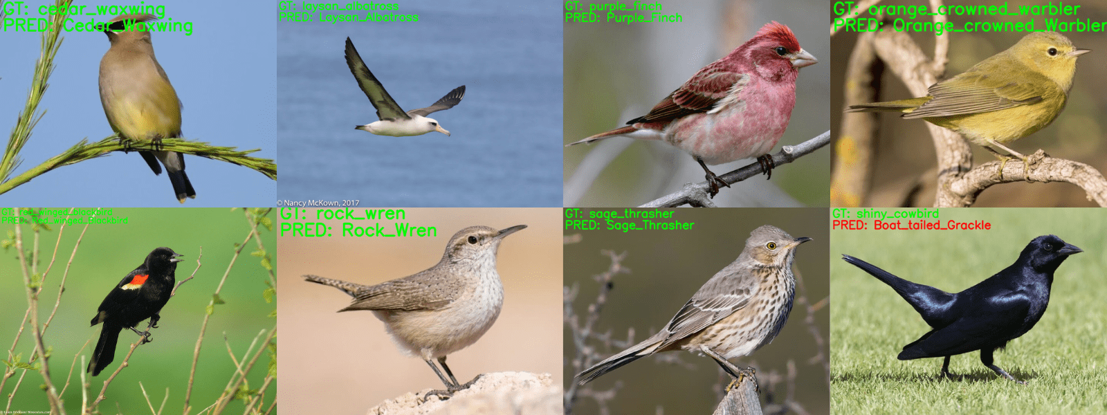
The results are really good but not perfect. The model made mistake in predicting the class of one of the birds. It is detecting the Shiny Cowbird as Boat Tailed Grackle.
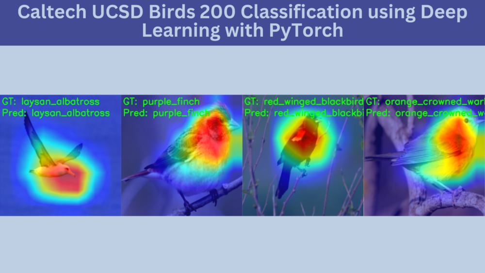
Before we dig further into the reason, we will run the cam.py script to visualize the class activation maps. This will give us a good idea of which parts of a bird the model focuses on.
python cam.py
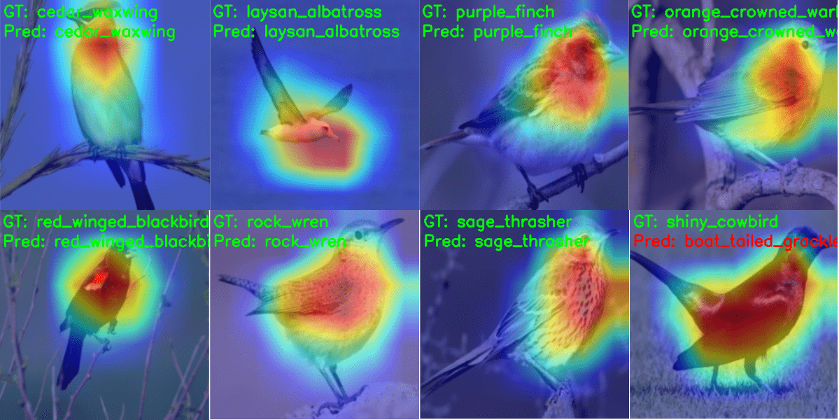
Most of the time the model trained on the Caltech UCSD Birds Classification is focusing on either the neck or the wing of the bird. For example, for the Red Winged Blackbird, most of the focus is centered around the red patch of the wing. But in the case of the Albatross, it seems to be the beak.
For the Shiny Cowbird, the model focuses on almost the entire body and predicts it as a Boat Tailed Grackle. Here, is a comparison between the two.
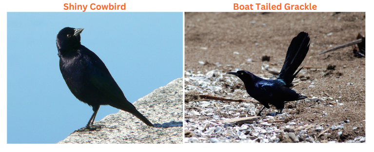
It does not seem fair to blame the model entirely here. The birds look almost exactly the same.
Further Experiments
Here are a few pointers for further experiments on the datasets.
- Trying out the good old ResNet50 which performs pretty well on a variety of datasets.
- Training larger models like EfficientNetB4 or ResNet101.
- Using other data augmentations to avoid overfitting and training longer.
If you try out any of the above experiments, do share your observations in the comment section. I am pretty sure they will be interesting to follow.
Summary and Conclusion
In this article, we trained an EfficientNetB1 model on the Caltech UCSD Birds Classification dataset. The dataset proved to be challenging considering the distinct features each bird possesses. After training, we conducted inference experiments and visualized the class activation maps also. This gave us more insights into where the model was failing. I hope that this article was worth your time.
If you have any doubts, thoughts, or suggestions, please leave them in the comment section. I will surely address them.
You can contact me using the Contact section. You can also find me on LinkedIn, and X.

1 thought on “Caltech UCSD Birds 200 Classification using Deep Learning with PyTorch”