Wheat Detection using Faster RCNN and PyTorch

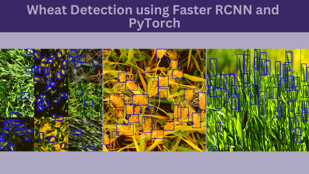
Needless to say, wheat as a crop is an integral part of agriculture. Analyzing their growth and health can be a challenge owing to the crop’s variety and diversity. But deep learning, especially, object detection can help with this. We can detect wheat heads using deep learning based object detection techniques. This in turn will make the analysis of the crop much faster. So, in this post, we will be using PyTorch and Faster RCNN for wheat head detection.

There may arise a question, “why do we need to detect wheat or wheat head using deep learning and object detection”? We will answer this question in a later part of the post and try to analyze its importance.

Before that, let’s sort out the points that we will cover in this post:

• We will start with a discussion of the dataset and the objective of this project.
• Then we will move on to discuss the codebase (a GitHub repository) that we will use to train the Faster RCNN model.
• Next, we will cover the training of the model and the analysis of the results.
• After that, we will use the Faster RCNN model which has been trained on the wheat detection dataset for inference.
• Finally, we will finish the post by discussing some future possibilities of this project.

Let’s jump into the details of the post now.

Why is Wheat Detection Important?

Wheat detection is more commonly known as wheat head or wheat spike detection. It is the process of detecting the wheat head (spikes) at the top of the wheat crop.

In fact, the process of wheat head detection (deep learning or not) is so important that there are several competitions out there to get the best solutions.

But again, the question arises. Why is the detection of the wheat head or wheat spike so important?

• As wheat is a global crop, it is grown in a lot of countries. As such there are several varieties of wheat all over the world. Scientists try to understand the crop production process for better yield.
• Detecting wheat heads can lead to the estimation of the size and density of different varieties.
• This can also lead to the analysis of the health and maturity of the wheat heads and in turn the wheat crop.

What Makes Wheat Head Detection Difficult?

All the varieties throughout the world are one of the major problems. Even with state-of-the-art object detection algorithms like YOLO and Faster RCNN, it is a challenging problem to solve.

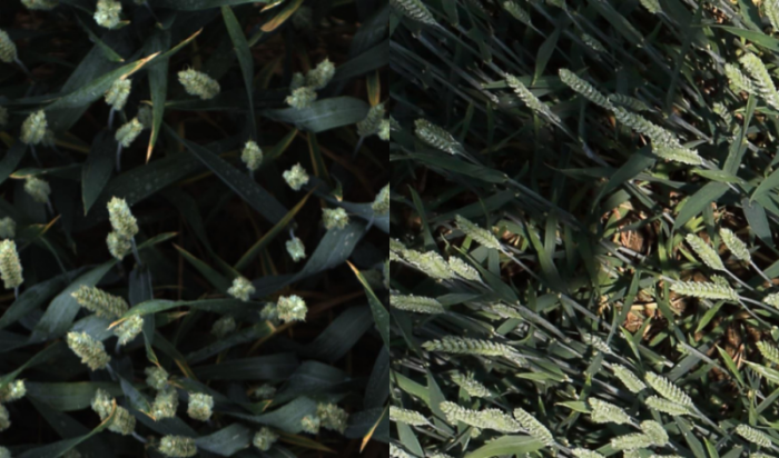
For instance, take a look at the following images.

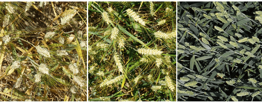
All the above images are from the same dataset, yet they appear so different. The colors, density of the crop, lighting, and the country which the wheat crop originates from can make the detection process particularly challenging.

This means that we need a pretty varied dataset for this task. To get more information on this, we can take a look at the dataset that we will use to train the Faster RCNN model for wheat detection.

The Wheat Detection Dataset

In this post, we will use the wheat detection dataset from Kaggle’s 2020 Global Wheat Detection competition. This features more than 3000 images of wheat heads and plants from different countries. The training dataset contains images from France, UK, Switzerland, and Canada.

The codebase that we will be using accepts the detection label files in XML format. But the competition dataset on Kaggle provides a CSV file containing the labels and bounding box information.

To tackle this, I have already prepared the XML labels of the images and also split the dataset into a training and a validation set. The test set remains intact as it was in the original set.

You can visit the following link to get the dataset.

• Global Wheat Detection 2020 Train/Valid/Test Split

The current dataset contains 3205 training images and 167 validation images. The train_imgs and valid_imgs directories contain the images and the train_labels and valid_labels contain the XML files.

For reference, the following is the structure of the directory after downloading and extracting the zip file.

.
├── test
├── train_imgs
├── train_labels
├── valid_imgs
└── valid_labels

The test directory contains the 10 test images that came with the original dataset.

For now, you may go ahead and download the dataset. After discussing the code base, we will see how to structure everything in the project directory.

The Faster RCNN Codebase

We will use the Faster RCNN training pipeline repository code for training the Faster RCNN model for wheat detection.

I have been developing the repository for the past several months. This has some nice utilities like:

• Several COCO pretrained models and ImageNet pretrained backbones with Faster RCNN head.
• Models that can run in real-time.
• Auto-logging to local storage, and Weights&Biases also.
• COCO evaluation metric support as well.

All of this will make our life much easier.

Download Code

You can go ahead and clone the repository.

git clone https://github.com/sovit-123/fasterrcnn-pytorch-training-pipeline.git

Before installing the requirements, I would recommend installing PyTorch using the Conda command according to your hardware.

conda install pytorch==1.12.0 torchvision==0.13.0 torchaudio==0.12.0 cudatoolkit=11.6 -c pytorch -c conda-forge

Next, install the remaining requirements using the following command.

pip install -r requirements.txt

If you are using Windows, check the following guideline to properly install pycocotools.

• Setup on Windows

This is all we need for the setup.

Project Directory Structure

Following is the project directory structure.

.
├── fasterrcnn-pytorch-training-pipeline
│   ├── data
│   ├── data_configs
│   │   ...
│   │   └── wheat_2020.yaml
│   ├── docs
│   │   ├── upcoming_updates.md
│   │   └── updates.md
│   ├── example_test_data
│   ├── models
│   │   ├── create_fasterrcnn_model.py
│   │   ├── fasterrcnn_convnext_small.py
│   │   ...
│   │   └── model_summary.py
│   ├── notebook_examples
│   │   ...
│   │   └── visualizations_wheat_detection.ipynb
│   ├── outputs
│   │   ├── inference
│   │   └── training
│   ├── torch_utils
│   │   ...
│   │   └── utils.py
│   ├── utils
│   │   ...
│   │   └── validate.py
│   ├── _config.yml
│   ├── create_submission.ipynb
│   ├── datasets.py
│   ├── eval.py
│   ├── inference.py
│   ├── inference_video.py
│   ├── __init__.py
│   ├── requirements.txt
│   ├── run.sh
│   ├── submission.csv
│   └── train.py
└── input
    ├── inference_data
    │   └── images
    ├── test
    │   ├── 2fd875eaa.jpg
        ...
    │   └── f5a1f0358.jpg
    ├── train_imgs [3205 entries exceeds filelimit, not opening dir]
    ├── train_labels [3205 entries exceeds filelimit, not opening dir]
    ├── valid_imgs [167 entries exceeds filelimit, not opening dir]
    ├── valid_labels [167 entries exceeds filelimit, not opening dir]
    └── sample_submission.csv

34 directories, 85 files

• The fasterrcnn-pytorch-training-pipeline is the cloned repository. There are four files here that we are the most interested in. They are the wheat_2020.yaml, train.py, inference.py, and inference_video.py. Subsequently, we will use each of these.
• The input directory contains the wheat detection dataset just in the format we discussed in one of the previous sections.

Please note that we will not go into the details of the code files. The codebase is quite large. Our main aim here is to carry out several training experiments and analyze the results. However, you are free to explore the Faster RCNN Training Pipeline repository to understand it better.

Downloading the zip file that is available with this post will provide you with the trained model (best weights) and the inference data. You can use this if you just want to run inference. Before that, please make sure to set up the directory in the above structure.

Wheat Detection using Faster RCNN MobileNetV3 Large FPN Model

Without any further delay, let’s jump into the interesting parts. The training, testing, and inference of the object detection models for wheat detection.

The Wheat Dataset YAML File

One of the mandatory requirements before we can start the training is the dataset YAML file. This YAML file contains all the information about the dataset. We need it during the training.

The YAML file information for the wheat detection dataset is inside data_configs/wheat_2020.yaml.

# Images and labels direcotry should be relative to train.py
TRAIN_DIR_IMAGES: '../input/train_imgs'
TRAIN_DIR_LABELS: '../input/train_labels'
VALID_DIR_IMAGES: '../input/valid_imgs'
VALID_DIR_LABELS: '../input/valid_labels'

# Class names.
CLASSES: [
    '__background__',
    'Wheat'
]

# Number of classes (object classes + 1 for background class in Faster RCNN).
NC: 2

# Whether to save the predictions of the validation set while training.
SAVE_VALID_PREDICTION_IMAGES: True

It contains the paths to the training and validation image folders, as well as the label folders. We also provide the class name information. One important point to note here is that the class name in this file should match what is present inside the XML files.

Along with that, we also provide the number of classes in this file. This should equal the total number of object classes in addition to the background class. So, in this case, the number of classes is 2.

Training Faster RCNN MobileNetV3 Models

We have all the necessities in place to start the training. For the wheat detection using Faster RCNN, we will fine-tune the Faster RCNN MobileNetV3 Large FPN model. In total, we will carry out four experiments. They are.

• Training Faster RCNN MobileNetV3 Large FPN model on the wheat detection dataset without any augmentations.
• Training the Faster RCNN model with mosaic augmentation.
• Faster RCNN wheat detection training without mosaic but with color and blur augmentations.
• Training the Faster RCNN model with all the augmentations.

All the training, testing, and inference experiments shown here were performed on a machine with:

• 10 GB RTX 3080 GPU
• 10th generation i7 CPU
• 32 GB DDR4 RAM

Let’s get into the training experiments now.

Faster RCNN MobileNetv3 Large FPN Training without Any Augmentations

To start the training without any augmentations, execute the following command in the terminal within the fasterrcnn-pytorch-training-pipeline directory.

python train.py --model fasterrcnn_mobilenetv3_large_fpn --data data_configs/wheat_2020.yaml --epochs 40 --no-mosaic --name fasterrcnn_mobilenetv3_large_fpn_noaug_40e --seed 42

The following are the command line arguments that we use here:

• --model: Name of the model that we want to use. In this case, we are using the COCO pretrained model.
• --data: This flag accepts the path to the dataset YAML file.
• --epochs: Number of epochs to train for.
• --no-mosaic: This is a boolean flag indicating that we don’t want to use mosaic augmentation.
• --name: We can give a comprehensive project name when executing the training command. All the results will be stored in this directory under outputs/training path.
• --seed: Although the training applies a seed value during training, we can also provide a seed manually for reproducibility.

If you are running the experiments on your own, it may take a while for the training to finish.

For this training, the best mAP (on the validation set) was on epoch 32. It was 46.21 mAP.

Average Precision  (AP) @[ IoU=0.50:0.95 | area=   all | maxDets=100 ] = 0.46219226325998325
Average Precision  (AP) @[ IoU=0.50      | area=   all | maxDets=100 ] = 0.8847548283407588
Average Precision  (AP) @[ IoU=0.75      | area=   all | maxDets=100 ] = 0.4373239831531729
Average Precision  (AP) @[ IoU=0.50:0.95 | area= small | maxDets=100 ] = 0.22314134508586306
Average Precision  (AP) @[ IoU=0.50:0.95 | area=medium | maxDets=100 ] = 0.4857252002861627
Average Precision  (AP) @[ IoU=0.50:0.95 | area= large | maxDets=100 ] = 0.5222265758416728
Average Recall     (AR) @[ IoU=0.50:0.95 | area=   all | maxDets=  1 ] = 0.016722548197820618
Average Recall     (AR) @[ IoU=0.50:0.95 | area=   all | maxDets= 10 ] = 0.15101983794355966
Average Recall     (AR) @[ IoU=0.50:0.95 | area=   all | maxDets=100 ] = 0.5276334171556301
Average Recall     (AR) @[ IoU=0.50:0.95 | area= small | maxDets=100 ] = 0.3063172043010753
Average Recall     (AR) @[ IoU=0.50:0.95 | area=medium | maxDets=100 ] = 0.5526668795911849
Average Recall     (AR) @[ IoU=0.50:0.95 | area= large | maxDets=100 ] = 0.5855263157894737

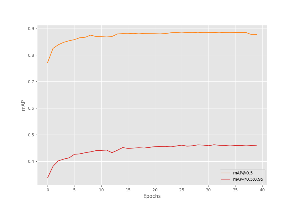
As we can clearly see, the mAP starts to dip just before the training ends. Most probably, training any longer would lead to overfitting.

Faster RCNN MobileNetv3 Large FPN Training with Color and Blur Augmentations

The color and blur augmentations that we will use here are already defined in utils/transforms.py file. They are:

• MotionBlur
• Blur
• RandomBrightnessContrast
• ColorJitter
• RandomGamma
• RandomFog
• MedianBlur

All these augmentations are applied using the Albumentations library. But why do we need to apply these augmentations?

Recall that when we were discussing how color, variety, and conditions specific to locations can affect the training of an object detection model for wheat head detection.

If we can show the model enough variety by applying all these augmentations, perhaps it will learn better. And it will be able to detect the wheat heads in different conditions. This is one of the major reasons to train the Faster RCNN model for wheat detection with all the augmentations.

Following is the training command.

python train.py --model fasterrcnn_mobilenetv3_large_fpn --data data_configs/wheat_2020.yaml --epochs 40 --no-mosaic --use-train-aug --name fasterrcnn_mobilenetv3_large_fpn_trainaug_40e --seed 42

Here are the best validation mAP results during training for the best epoch (epoch 36).

Average Precision  (AP) @[ IoU=0.50:0.95 | area=   all | maxDets=100 ] = 0.46437972689325324
Average Precision  (AP) @[ IoU=0.50      | area=   all | maxDets=100 ] = 0.8854726765032528
Average Precision  (AP) @[ IoU=0.75      | area=   all | maxDets=100 ] = 0.4369478807276368
Average Precision  (AP) @[ IoU=0.50:0.95 | area= small | maxDets=100 ] = 0.22131277443592978
Average Precision  (AP) @[ IoU=0.50:0.95 | area=medium | maxDets=100 ] = 0.48911422605495347
Average Precision  (AP) @[ IoU=0.50:0.95 | area= large | maxDets=100 ] = 0.5352173288475779
Average Recall     (AR) @[ IoU=0.50:0.95 | area=   all | maxDets=  1 ] = 0.016848281642917014
Average Recall     (AR) @[ IoU=0.50:0.95 | area=   all | maxDets= 10 ] = 0.15255658005029338
Average Recall     (AR) @[ IoU=0.50:0.95 | area=   all | maxDets=100 ] = 0.5297429449566918
Average Recall     (AR) @[ IoU=0.50:0.95 | area= small | maxDets=100 ] = 0.30510752688172044
Average Recall     (AR) @[ IoU=0.50:0.95 | area=medium | maxDets=100 ] = 0.5552060044714149
Average Recall     (AR) @[ IoU=0.50:0.95 | area= large | maxDets=100 ] = 0.5875

The model reaches 46.43 mAP in this case.

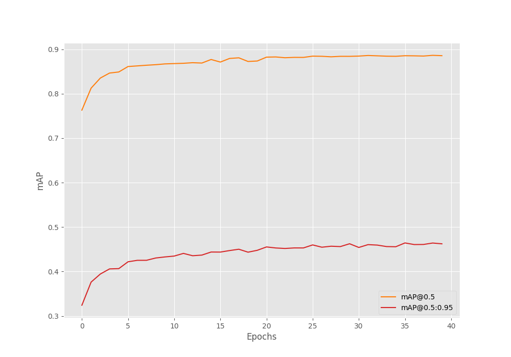
Interestingly, it looks like we can train the model for even longer in this case. Also, training with augmentations helped the model reach a higher mAP without overfitting.

Faster RCNN MobileNetv3 Large FPN Training with Mosaic Augmentation

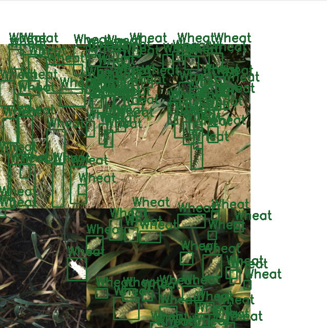
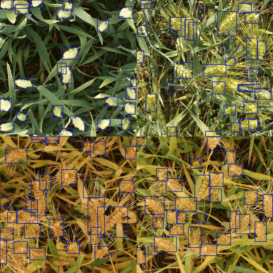
In mosaic augmentation, four images are stitched together. This helps to put more context in a single image, train with smaller images (as images are resized and cropped), and makes each image slightly difficult to learn as well.

The Faster RCNN training repository that we are using for wheat detection supports mosaic augmentation and applies it by default. For reference, the following is an example of a mosaic-augmented image that goes into the neural network.

The following is the command to train with mosaic augmentation.

python train.py --model fasterrcnn_mobilenetv3_large_fpn --data data_configs/wheat_2020.yaml --epochs 40 --name fasterrcnn_mobilenetv3_large_fpn_mosaic_40e --seed 42

The model was able to reach a maximum mAP of 24.28 on epoch 26.

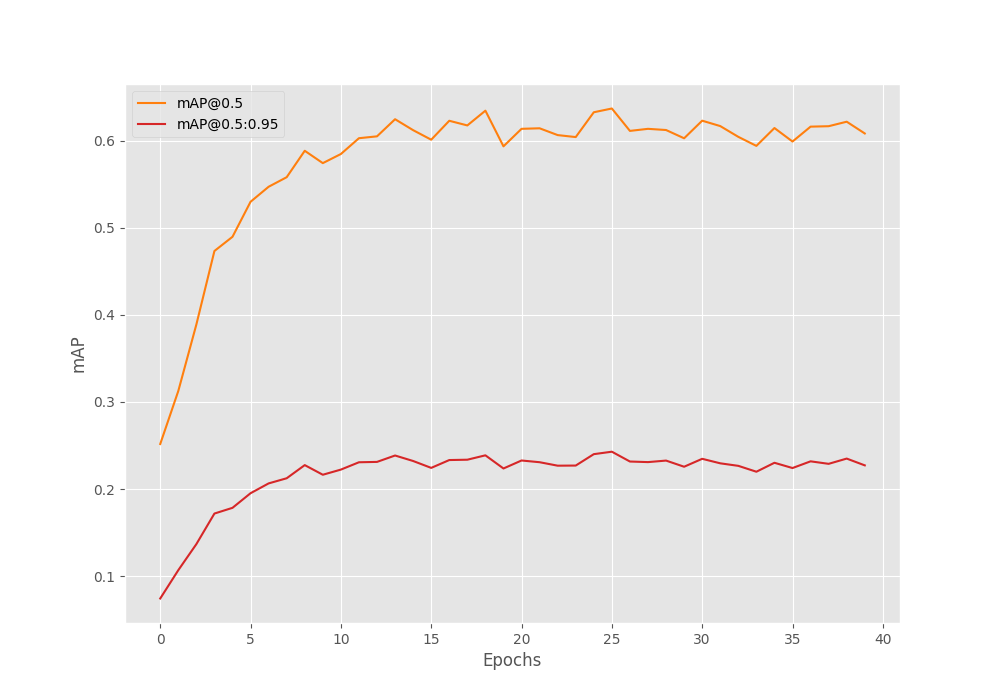
Average Precision  (AP) @[ IoU=0.50:0.95 | area=   all | maxDets=100 ] = 0.2428678932647114
Average Precision  (AP) @[ IoU=0.50      | area=   all | maxDets=100 ] = 0.6369417263134797
Average Precision  (AP) @[ IoU=0.75      | area=   all | maxDets=100 ] = 0.12355194070473341
Average Precision  (AP) @[ IoU=0.50:0.95 | area= small | maxDets=100 ] = 0.0724221664101825
Average Precision  (AP) @[ IoU=0.50:0.95 | area=medium | maxDets=100 ] = 0.26451922340385897
Average Precision  (AP) @[ IoU=0.50:0.95 | area= large | maxDets=100 ] = 0.2080252768772267
Average Recall     (AR) @[ IoU=0.50:0.95 | area=   all | maxDets=  1 ] = 0.010715283598770607
Average Recall     (AR) @[ IoU=0.50:0.95 | area=   all | maxDets= 10 ] = 0.09642358200614697
Average Recall     (AR) @[ IoU=0.50:0.95 | area=   all | maxDets=100 ] = 0.33744062587314894
Average Recall     (AR) @[ IoU=0.50:0.95 | area= small | maxDets=100 ] = 0.215994623655914
Average Recall     (AR) @[ IoU=0.50:0.95 | area=medium | maxDets=100 ] = 0.3531778984350048
Average Recall     (AR) @[ IoU=0.50:0.95 | area= large | maxDets=100 ] = 0.2875

There were also a lot of fluctuations in the mAP graph as we can see. This is most probably because the model is not well-suited for mosaic augmentation. The pretrained model (on COCO dataset) was never trained with mosaic augmentation. So, it is less likely that it will perform any better when fine tuning.

Faster RCNN MobileNetv3 Large FPN Training with All Augmentations

For the final Faster RCNN wheat detection experiment, let’s train with all the augmentations.

We include all the training augmentations using albumentations and mosaic augmentations also.

python train.py --model fasterrcnn_mobilenetv3_large_fpn --data data_configs/wheat_2020.yaml --epochs 40 --use-train-aug --name fasterrcnn_mobilenetv3_large_fpn_allaug_40e --seed 42

In this experiment, the model reached the maximum mAP of 25.15 on epoch 13.

Average Precision  (AP) @[ IoU=0.50:0.95 | area=   all | maxDets=100 ] = 0.2515069729679091
Average Precision  (AP) @[ IoU=0.50      | area=   all | maxDets=100 ] = 0.6696349967492324
Average Precision  (AP) @[ IoU=0.75      | area=   all | maxDets=100 ] = 0.1225353401488652
Average Precision  (AP) @[ IoU=0.50:0.95 | area= small | maxDets=100 ] = 0.08314289003940148
Average Precision  (AP) @[ IoU=0.50:0.95 | area=medium | maxDets=100 ] = 0.2711438018405023
Average Precision  (AP) @[ IoU=0.50:0.95 | area= large | maxDets=100 ] = 0.20890733962530217
Average Recall     (AR) @[ IoU=0.50:0.95 | area=   all | maxDets=  1 ] = 0.011371891589829562
Average Recall     (AR) @[ IoU=0.50:0.95 | area=   all | maxDets= 10 ] = 0.0967309304274937
Average Recall     (AR) @[ IoU=0.50:0.95 | area=   all | maxDets=100 ] = 0.35474993014808603
Average Recall     (AR) @[ IoU=0.50:0.95 | area= small | maxDets=100 ] = 0.2502688172043011
Average Recall     (AR) @[ IoU=0.50:0.95 | area=medium | maxDets=100 ] = 0.36935483870967745
Average Recall     (AR) @[ IoU=0.50:0.95 | area= large | maxDets=100 ] = 0.27039473684210524

Taking a look at the mAP graph reveals one more observation.

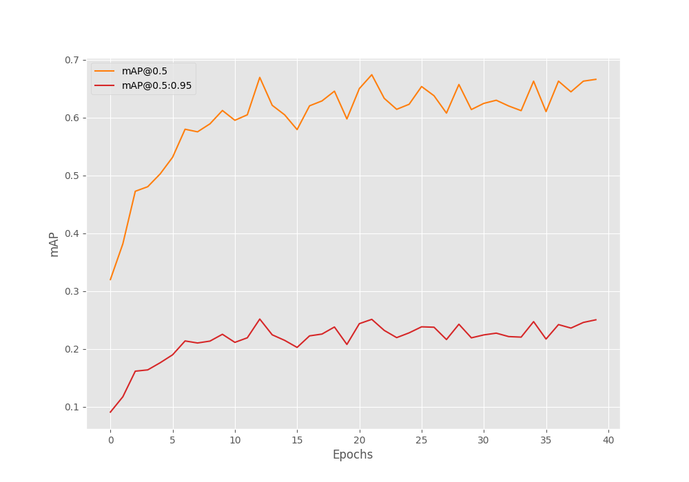
Although the mAP did not reach any higher, the model does not seem to overfit just yet. Including all the augmentations makes the dataset much harder to learn. And most probably, we can train for much longer in this. Maybe that’s something you can play with and tell about your findings in the comment section.

Inference for Wheat Detection using the Trained Faster RCNN Model

Now, let’s run inference using the best-performing model that we have, the one with albumentations training augmentations.

Inference on Images

We will start by running inference on the test images that came with the original dataset. We can use the inference.py to do so.

python inference.py --weights outputs/training/fasterrcnn_mobilenetv3_large_fpn_trainaug_40e/best_model.pth --input ../input/test/ --no-labels

These are the command line arguments that we need to take care of:

• --weights: Path to the trained PyTorch model.
• --input: Directory containing the images.
• --no-labels: This tells the inference.py script to hide the labels. As we have only one class in this dataset, we do not need to clutter the detections with the class name information.

Following are some of the outputs out of the 10 images from the test set.

The model is performing pretty well here. In fact, in the first image, it is detecting a wheat head at the bottom left which is barely visible. But at the same time, it is detecting some of the stem parts of the crop as the wheat head.

To assess the model better, let’s run inference on some unseen images from the internet. These images are available for download with this post. You may also run inference on your own images.

python inference.py --weights outputs/training/fasterrcnn_mobilenetv3_large_fpn_trainaug_40e/best_model.pth --input ../input/inference_data/images/ --no-labels

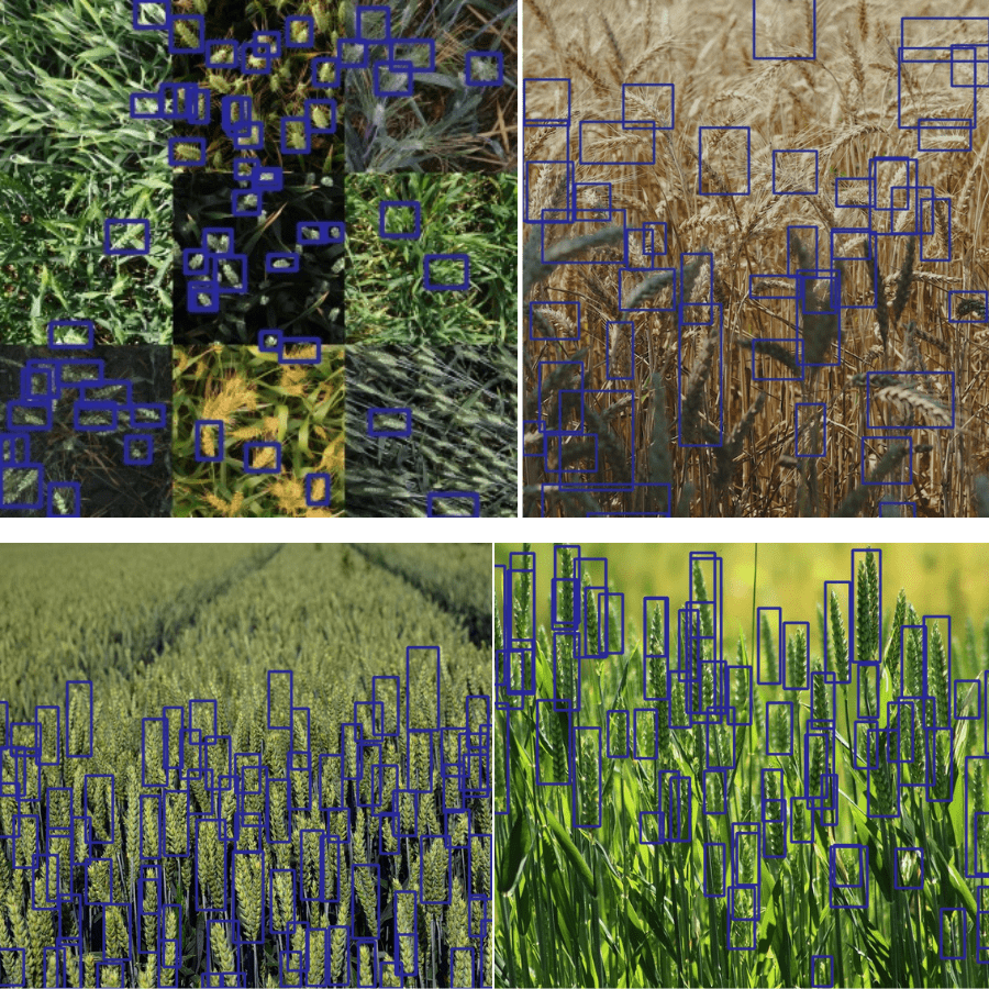
A few of the limitations of the model are visible here. As we move away from images that are not similar to the training data, the performance starts to worsen. Going in a clockwise direction, the first image shows a collage of 6 very small images in the top view. Here, the model is not able to detect all the wheat heads in the second image in the third row.

Coming to the second image, the model is missing out on a lot of wheat heads which are clearly visible. Though, the detections of wheat heads in the third image are pretty good.

Faster RCNN Wheat Head Detection on Video

For one final test, we will try out detections on a video. This time, we will use the inference_video.py script.

python inference_video.py --weights outputs/training/fasterrcnn_mobilenetv3_large_fpn_trainaug_40e/best_model.pth --input ../input/inference_data/videos/video_1.mp4 --no-labels --show

As you may see, the detections from the model are not very good here. This shows the limitations of moving objects. Further, it is detecting the tree as a wheat head in many of the frames as well.

Future Possibilities

When running inference, we observed that the Faster RCNN MobileNetV3 FPN model is not performing very well on moving objects and top-view images. There are a few steps we can take to improve the detection performance.

• The simplest step that we can take is to train a larger model. We can try training a Faster RCNN model with the ResNet50 backbone.
• Next, we can add images of wheat heads in the training set that have been captured by a drone flying over wheat fields. This will add ample top-view images.
• We can also add more blur augmentations so that the model learns the features of blurry and moving objects much better.

Summary and Conclusion

In this blog post, we trained a Faster RCNN MobileNetV3 Large FPN model for detecting wheat heads. We trained several models with different augmentations techniques. After running inference, we go to know the limitations of the model and where it is failing. We also discussed some points on improving the detection performance. I hope that this blog post was worthwhile for you.

If you have any doubts, thoughts, or suggestions, please leave them in the comment section. I will surely address them.

You can contact me using the Contact section. You can also find me on LinkedIn, and Twitter.