
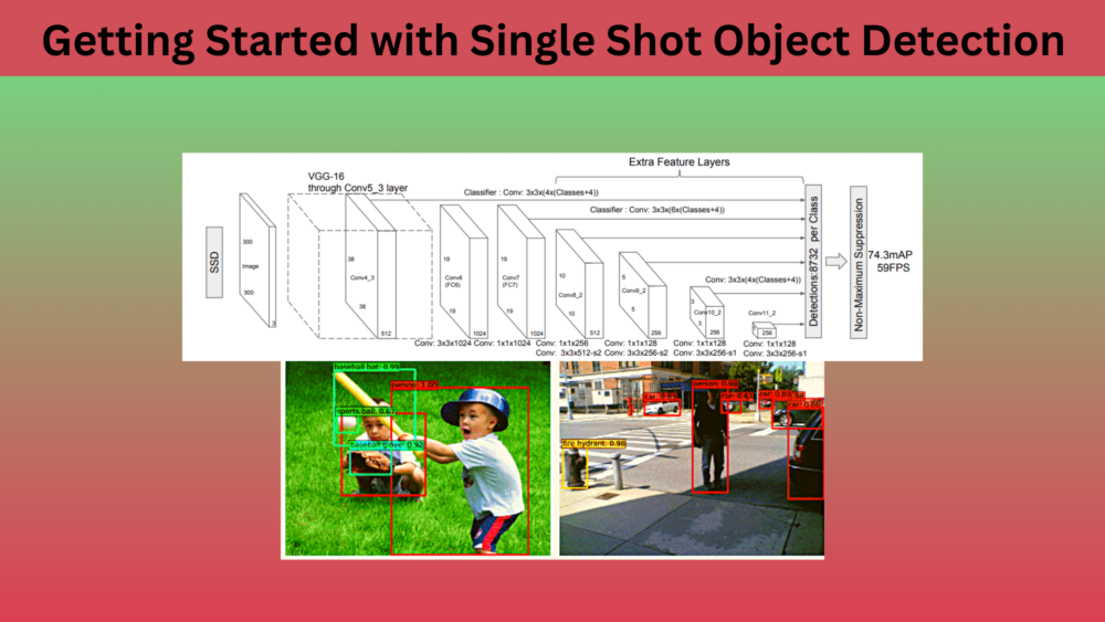
Object detection is one of the most practical aspects of computer vision. It can help solve many problems. These include, but are not limited to disease detection in plants and humans, autonomous driving of vehicles, security & surveillance, and many more. In this blog post, we will discuss the Single Shot Object Detection Model. This involves going into the details of the SSD paper (Single Shot MultiBox Detector) by Liu et al.
In the last few years, single shot object detection models have come a long way. Starting from the very first version of YOLO to SSD, and the many YOLO object detection detection models that followed. The list of single shot object detection models is quite huge now in the deep learning world.
For beginners, it becomes quite difficult to get into the field of object detection in deep learning. The SSD (Liu et al) and the YOLO v1 (Redmon et al) models are some of the best papers to start understanding single shot object detectors. For now, we will start with the SSD paper.

In this post, we will be discussing the following points from the paper.
- How is SSD different from the previous object detection models that use deep learning approach? What does the SSD network architecture look like?
- A short discussion on default boxes (or prior boxes) in SSD.
- What does SSD do differently in comparison to YOLO and Faster RCNN models?
- The loss function that is used to train SSD.
- The training parameters and criteria.
- What are the results and benchmarks on the Pascal VOC dataset?
This post should give you a good idea of how SSD is different from other object detection models.
The Single Shot MultiBox Object Detection Model
The Single Shot MultiBox Object Detection (SSD for short) model was published by Wei Liu et al in 2015. After that, it has had several updates and the current version on arxiv is version 5.
It was the first deep learning based object detector to give both, real-time speed and state-of-the-art accuracy.
Prior to SSD, YOLOv1 also was able to achieve real-time speed. But the accuracy was not that good. To get state-of-the-art speed and accuracy, SSD used the following techniques:
- Like YOLOv1, SSD is also a single-stage detector. But instead of dividing an image into a 7×7 grid and detecting 2 objects per grid, SSD adopts the method of default boxes. After a few years, we know these as anchor boxes in deep learning and object detection.
- Moving away from the two-stage detectors like Faster RCNN, SSD adopted the concept of a single deep neural network for detection and classification.
- All the detection of the boxes and classification takes place within a single deep neural network, completely end-to-end.
- For each default box, the SSD network produces prediction scores for all the categories in a dataset.
- The SSD model combines predictions from feature maps of different sizes. This helps in detecting objects of varying sizes.
Among the above, perhaps the most important change is adopting a single-stage detection strategy. Unlike Faster RCNN, it neither has a proposal generation network nor does it do ROI (Region Of Interest) pooling. Still, it was able to achieve state-of-the-art accuracy of 74.3 mAP running at 59 FPS on NVIDIA Titan X GPU. We will uncover how it does that further in the article.
The Single Shot Detection Network Architecture
The SSD network introduced in the paper has two variants, SSD300 and SSD512. The SSD300 accepts images of 300×300 resolution and SSD512 accepts 512×512 resolution images.
Although there is a difference in the input size, the underlying architecture does not change. So, following this, let’s understand the important bits of the SSD model architecture.
The SSD model is a feed-forward network that outputs a set of bounding boxes and the scores for each of the classes. The base layers or more commonly known as the backbone of the network can be any image classification model, although with one catch. We do not include the final classification layers of that network. We only include the feature extraction layers.
The most common SSD300 is with VGG16 backbone. But we can use any model for feature extraction, be it ResNet18, ResNet34, or even EfficientNet models as of now.
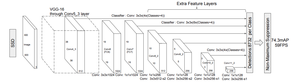
Figure 2 shows the complete SSD architecture along with the backbone layers and the detection layers as well. As you may see, it uses the VGG16 model as the backbone. But that’s not all. A few extra feature extraction layers are also added after the base VGG16 layers.
These extra layers at the end (along with the layers that do the detection) comprise the auxiliary part of the model. Now, what does this auxiliary structure help us achieve?
This essentially encompasses three important factors of the SSD model which made it so successful (and still pretty good, to be fair). These include:
- Multi-scale feature map for detections.
- Convolutional predictors for detection.
- Default boxes and their aspect ratios.
We will tackle the above three points in the next few sections.
Multi-Scale Feature Maps for Detections
The SSD model combines detection results from multiple layers with different scales. That’s why the term multi-scale feature maps for detection.
Let’s take a closer look at the SSD model again.
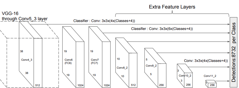
We can see that each of the convolutional layers has been named, such as Conv4_3, Conv6, and so on. Also, we can see the dimension of each of the feature maps. For example, Conv4_3 has a dimension of 38×38. Along with that, we can see a line from Conv4_3 to the final detection block.
Not only that. Observing the Conv4_3, Conv_7, Conv8_2, Conv9_2, Conv10_2, and Conv11_2 reveals a line from each of these to the final detection block. This indicates that the bounding box predictions from each of these layers are used in the final predictions. A total of 6 layers with different feature map resolutions are used to predict the 8732 bounding boxes and their scores.
For now, we will not go into the details of how it results in 8732 bounding boxes. We will dive into the depths of SSD in one of the future posts, where we will break down SSD to make it as simple as possible. Right now, there are two important points to remember.
- SSD predicts bounding box locations and their scores at six different layers.
- These layers result in feature maps with different resolutions (38×38 to 1×1) which in turn helps in multi-scale predictions and detection of objects of varying sizes.
Convolutional Predictors for Detections
As discussed above, each of the multi-scale feature maps is responsible for producing detection predictions and scores. For the detections, the outputs are not directly bounding boxes. Rather, they are offsets to the default box coordinates.
Let’s say that a feature map is of shape m x n with p channels. It is associated with a 3 x 3 kernel with p channels. This kernel is applied to each m x n location of the feature map, outputting the score and offsets for the default boxes.
The detection predictions are relative to a default box.
This brings us to the third most important post. It is default boxes.
Default Boxes
Default boxes, otherwise known as prior boxes, or more commonly as anchor boxes nowadays.
The SSD network used default boxes which are similar to anchor boxes in Faster RCNN. SSD associates each feature map cell where detection happens (the 6 that we discussed above) with a set of default bounding boxes.
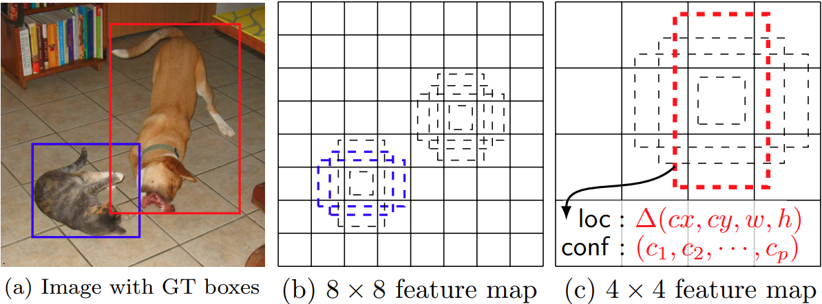
Let’s try to understand this by looking at figure 4. As you may see, the feature maps are divided into 8×8 and 4×4 grids. Each grid (grid cell location) associates itself with 4 default boxes of different aspect ratios. For each of the default boxes, the Single Shot Detection model predicts box shape offsets and confidence scores for each category.
The model predicts 4 offset values for each location as we see from the above image. Let’s take the example of a particular feature map. Say, there are c object classes (excluding the background). There are 4 offset values for each location. Then, if the size of the feature map is m x n, then the total number of outputs for that feature map will be (c + 4)kmn, where k is the total number of boxes at each grid cell location.
Obviously, these are a lot of outputs and it is kind of difficult to visualize this without a practical example. We will not dive into any more complicated diagrams in this post. It’s better to dedicate an entire post to Single Shot Detection architecture and write it from scratch to understand it better.
Box Predictions
To train the detection head of the Single Shot Detection model, we predict the offsets from the default boxes. These are the center offsets and the width and height offsets to the default box \(d\).
Let’s call the center coordinates \(cx, cy\), and width & height as \(w, h\). Let the ground truth box be \(g\).
Now, the offsets can be calculated using the following formula:
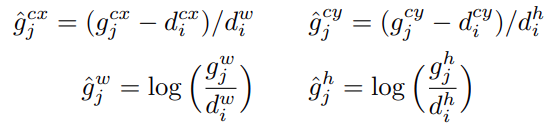
Here, \(g\) indicates the ground truth box. The above formula becomes important as we move towards the loss function that is used to train the SSD model.
Before Moving Further
There are a few things that we did not touch upon in detail in the above sections. They are:
- Default box aspect ratios
- Default box scales
- The number of box outputs per detection feature map
- And of course, how they all come together to build the SSD model
We will discuss all of this while building SSD from scratch in one of the future posts.
The Loss Function for Single Shot Detection
The SSD model outputs the location predictions and the confidence scores during training. So, the loss function is a combination of the localization loss and the confidence loss.
The localization loss is a smooth L1 loss.
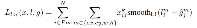
In the above formula, \(l\) is the predicted box, and \(g\) is the ground truth box.
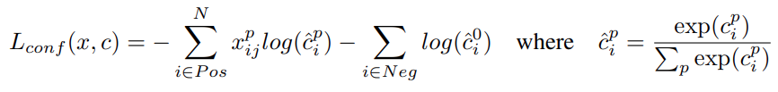
For the confidence loss, SSD uses the softmax loss over multiple class confidences \(c\).
Combining the above two losses gives us the final loss.
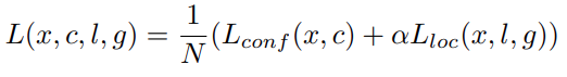
Here, \(N\) is the number of matched default boxes, and \(\alpha\) is a weight value for the localization loss.
Training Criteria
The VGG16 model as per the paper is one that has already been trained on the ImageNet dataset. So, for fine-tuning the Single Shot Object Detection model, the authors use the following strategy.
| Optimizer | SGD |
| Initial learning rate | 0.001 |
| Momentum | 0.9 |
| Weight Decay | 0.005 |
| Batch size | 32 |
As per the authors, every training starts with the above values but needs fine-tuning depending on the dataset.
For example, for the Pascal VOC 07+12 dataset, they train with a 0.001 learning rate for the first 60000 iterations. And for the next 20000 iterations, the learning rate is 0.0001.
You can find the details about other datasets and their hyperparameters in sections 3.1, 3.2, and 3.3 of the paper.
Benchmarks and Results for the Single Shot Object Detection Model
Let’s check some of the benchmark results after training the SSD model on the Pascal VOC dataset.
The following image shows the results in the Pascal VOC 2007 test dataset after training on different datasets for different models.
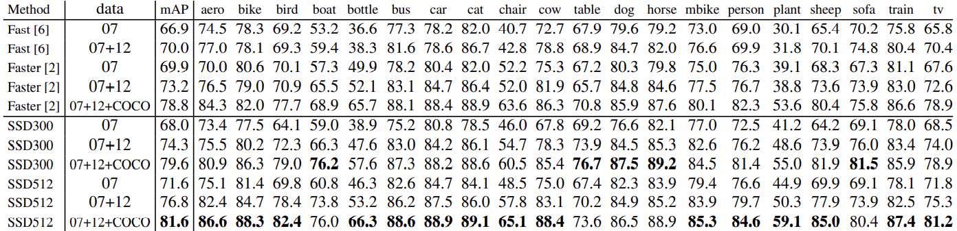
It is pretty clear that at the time of publication, Single Shot Object Detection models were able to beat Faster RCNN models. The best results are after training on Pascal VOC 2007 + 2012 + COCO dataset. With 81.6 mAP object detection metric, it was able to beat Faster RCNN.
What’s even more impressive is that SSD uses either an input size of 300×300 or 512×512, while Faster RNN used an input size of 600×600 for the above results.
Now, coming to some results on the Pascal VOC 2012 test set.
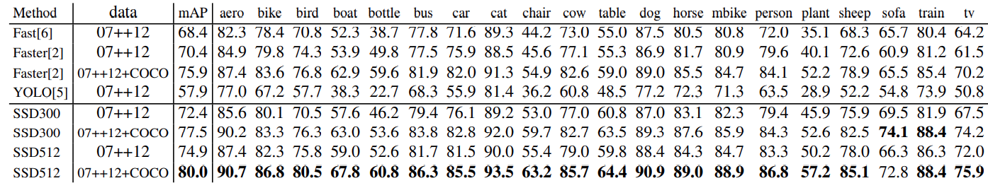
Here also, SSD is beating all the other models in terms of mAP. The most interesting part here is that, though both YOLO and SSD are real-time object detection models, SSD has almost 22 mAP more than YOLO.
Summary and Conclusion
In this post, we went through a few details, results, and benchmarks of the Single Shot Object Detection model. We covered most of the model architecture in a theoretical manner. One can get much more insights when writing the model from scratch, which we will do in a future post. I hope that this post is useful to you.
If you have any doubts, thoughts, or suggestions, please leave them in the comment section. I will surely address them.
You can contact me using the Contact section. You can also find me on LinkedIn, and X.
References

very well illustrated Single shot detection.
Thank you.