Saliency Maps in Convolutional Neural Networks

Convolutional neural networks (CNNs) have led to great improvement in computer vision. But a few questions have always bothered practitioners and researchers alike when using CNNs. Why does the neural network predict a particular label? What did it see in the image that led to a particular prediction? We can answer these questions through saliency maps. In this article, we will learn about saliency maps in convolutional neural networks.

Deep learning and neural networks have shown great capability in the field of computer vision. Image classification, object detection, image segmentation, and video analytics are some of the best examples. But understanding convolutional neural networks is still important. Mainly, when we want to interpret what a CNN sees. Saliency maps and the variations of the technique help us in this regard. We will understand some of the best methods in brief in this article.

What will you learn in this article?

In this article, we will have a brief overview of different saliency map techniques from different papers. This should give us a good idea of how different convolutional neural network interpretation methods work. Also, we will take a look at the different methods in detail in future posts.

• Introduction to Saliency Maps.
  • What are saliency maps?
• Different approaches to saliency maps as per different papers.
  • Deconvolutional Network Approach (Visualizing and Understanding Convolutional Networks, Zeiler and Fergus).
  • Gradient-Based Approach (Deep Inside Convolutional Networks: Visualising Image Classification Models and Saliency Maps, Simonyan et al.).
  • Guided Backpropagation Algorithm (Striving for Simplicity: The All Convolutional Net, Springenberg et al.).
  • Class Activation Mapping (CAM) Approach (Learning Deep Features for Discriminative Localization, Zhou et al.).
  • Grad-CAM (Grad-CAM: Visual Explanations from Deep Networks via Gradient-based Localization, Selvaraju et al.).

Note: You will get to learn about all the different approaches in brief in this article. In further articles, we will discuss all the methods with hands-on programming in detail, along with paper review and discussion

Also, if you wish, you may take a look at the previous article, Basic Introduction to Class Activation Maps in Deep Learning using PyTorch. Here, you will learn about a code-first approach to visualizing heat maps using PyTorch and ResNet18.

Introduction to Saliency Maps in Convolutional Neural Networks

First of all, you might be familiar with saliency maps or it may be a very new topic for you. If you are well familiar with the topic of saliency maps in convolutional neural networks, then I would love to hear your thoughts in the comment section. And if you are new to the topic, let us go through the topic together.

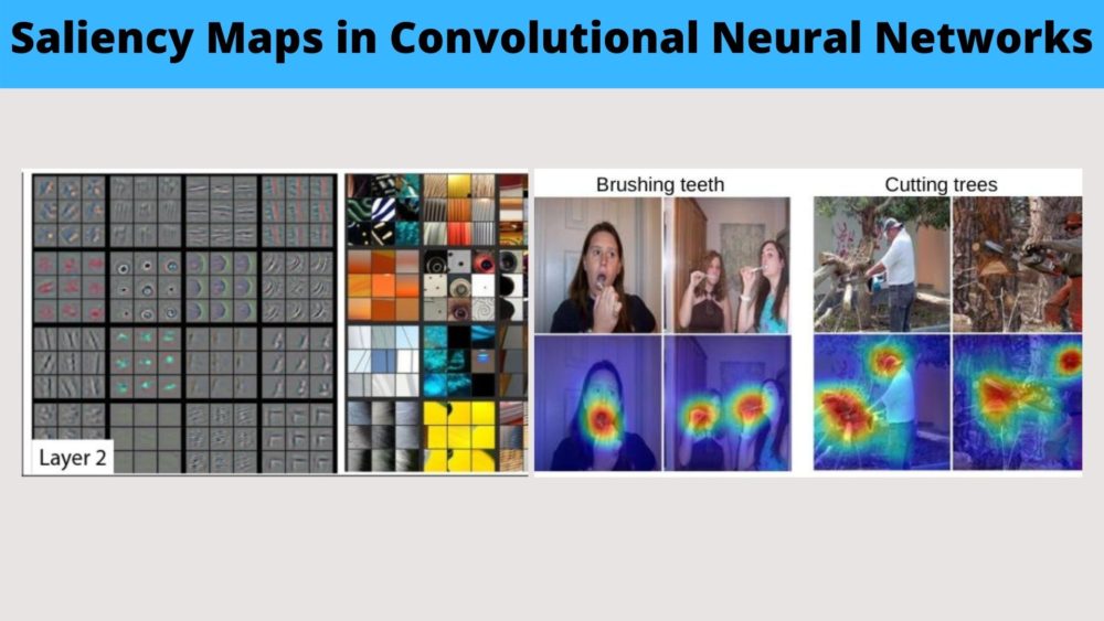
Let’s start by taking a look at the following image.

For us humans, it is pretty easy to know that it is a cat. But for convolutional neural networks, to classify it as a cat, they need to be trained on hundreds and thousands of cat images. Even then, there is a chance that convolutional neural networks might misclassify the image in some situations. And even when the neural network model classifies the image correctly, knowing which part of the image exactly led to the prediction will give us better insights.

This is where saliency maps in convolutional neural networks help.

What are Saliency Maps?

So, what are saliency maps?

Saliency maps are a visualization technique to gain better insights into the decision-making of a neural network. They also help in knowing what each layer of a convolutional layer focuses on. This helps us understand the decision making process a bit more clearly.

Saliency maps help us visualize where the convolutional neural network is focusing in particular while making a prediction. Suppose that we feed the above image of the cat to the model. And the model correctly predicts it as a cat.

What exactly led to that prediction? Is it the fur? Is it the eyes? Or is it the pointy ears of the cat? Saliency maps can provide answers to these questions with some good visualizations.

Generally, we visualize saliency maps as heatmaps overlayed on the original image. We can also visualize them as colored pixels concentrated around the area of interest of an object.

The following image will give you a pretty good idea.

Let’s now go over all the difference saliency map techniques.

Deconvolutional Network Approach

The decovnolutional network approach was proposed by Zeiler and Fergus in the paper Visualizing and Understanding Convolutional Networks.

This was one of the very first methods to understand the intermediate layer activities in convolutional neural networks. Till the publication of the paper, image classification networks had already started to perform well. But it was difficult to know why so. The authors try to create a novel visualization technique to answer the question.

Basically, they perform visualization with a deconvolutional network. Here, they try to map the intermediate layer visualizations of a neural network to the input. This helps in knowing which pattern led to the activation of the feature maps.

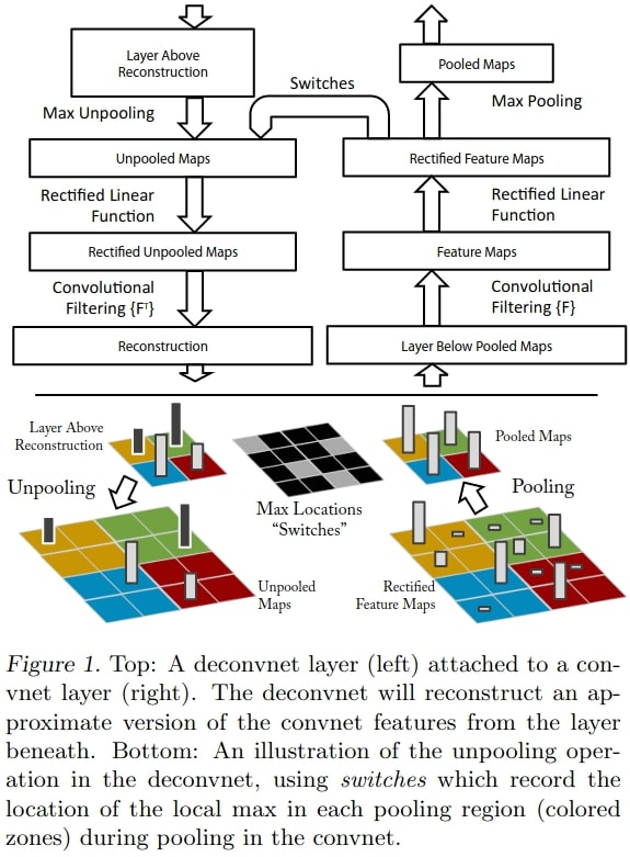
The above shows the deconvnet approach used by the authors in the paper.

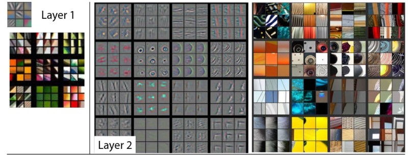
Figure 5 shows the feature maps along with the input space. The patterns in the features maps show which part causes high activation. We can see that initially (layers 1 and 2), edges and circular patterns cause most of the activations. If you take a look at Figure 2 in the paper, then you will notice that later layers are activated by more image-specific sophisticated features like tires of car and faces of dogs.

The paper contains a lot more detail which is difficult to contain in this introductory post. If you are interested, be sure to give the paper a read.

Gradient Based Approach for Saliency Maps

The gradient-based approach for saliency map visualization was introduced by Simonyan et al. in the paper Deep Inside Convolutional Networks: Visualising Image Classification Models and Saliency Maps.

In the paper, the authors address the visualization of image classification models. These models employ the Convolutional Neural Networks for learning the image features.

In fact, the authors explore two methods for saliency maps in the paper.

• The first method generates an image. This is a class model visualization technique learned by the classification convolutional network. Basically, we have a trained convolutional neural network and a class of interest that we provide to the trained network. Then the neural network’s visualization will consist of numerically generating the image.
• The second method consists of computing a class saliency map. This is image-specific class saliency visualization which shows which part of an image leads to the maximum class score.

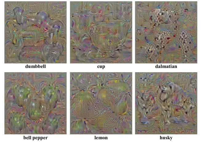
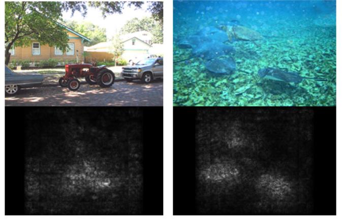
Figure 6 shows the numerically computed images based on the first method. These are learnt by the ConvNet and the ConvNet can also capture different class appearances for a single image.

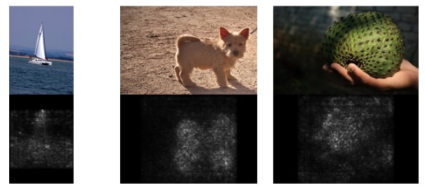
Figure 7 shows method 2 from the paper here. That is, class saliency map visualization. This shows the part of an image which leads to the maximum class score.

Guided Backpropagation Algorithm Approach

Springenberg et al. propose a new method for image recognition in the paper Striving for Simplicity: The All Convolutional Net.

They find that the max-pooling layers in convolutional neural networks can be replaced by convolutional layers. They propose an architecture consisting of convolutional layers only for image recognition. And because of the all convolutional net, they are also able to propose a new method of learned feature visualization using a variant of the deconvolution approach.

They build upon the work of Zeiler and Fergus who used deconvnet for activation feature visualization. In the process, they also find out that without max-pooling, the visualization of the discriminative features does not work very well when using deconvolutional network. This leads them to find a new way. The authors call their new method the guided backpropagation method.

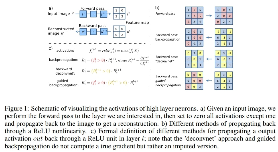
Figure 8 shows different methods of propagating back through ReLU non-linearity along with the guided backpropagation method.

The Steps for the Guided Backpropagation method

Let’s see what are the steps that the authors follow for the guided backpropagation approach using a “deconvnet”.

• We have a high-level feature map. The deconvnet inverts the data flow to the CNN. This data inversion flows from the current neuron activations to the image that we input.
• After the above step, only a single neuron is non-zero in the high level feature map.
• The final reconstructed image shows the parts of the input image that highly activates the neuron. This is the discriminative part of the image for the neuron.

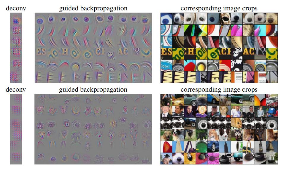
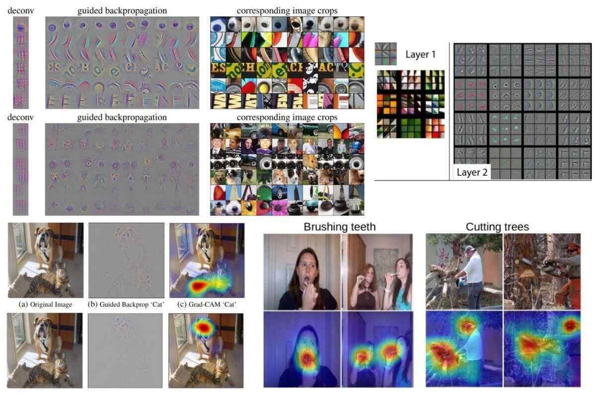
Figure 9 shows the visualizations from the learned all convolutional network using the guided backpropagation method. We can see that conv6 features are mostly activated because of edges, circles, and arcs. As we proceed to conv9, the activation features become more sophisticated. These are almost full images of faces of persons, dogs, and complete images of other objects as well.

Class Activation Mapping (CAM)

Zhou et al. introduce the method of class activation mapping the paper Learning Deep Features for Discriminative Localization. They also propose a modification to the global average pooling. This leads to the claim that even convolutional neural networks trained for image classification can have good localization capabilities.

They propose to visualize parts of an image that activate the convolutional neural network as heatmaps overlayed on the image.

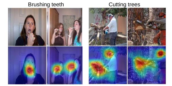
Figure 10 shows an example from the paper. When the authors combine the modification of the global average pooling along with their class activation mapping technique, they find something interesting. The model is able to both recognize the activity and also localize specific image regions which leads to the prediction of the class.

The authors use the term Class Activation Maps to refer to weighted activation maps generated by a CNN. These weighted activations lead to the prediction of a specific label for the image. If you are interested in the code, you can find the sample code from the paper here.

The following image will make things a bit more clearer.

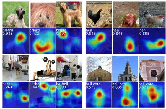
Thanks to class activation mapping, we can see in the above figure which parts of an image lead to the prediction of a specific class by the neural network. For example, the head of the dog, barbells in the gym, and the others as well.

If you want to get hands-on with class activation mapping using PyTorch, then please visit the previous post. I am sure you will learn something new.

Grad-CAM

In the paper Grad-CAM: Visual Explanations from Deep Networks via Gradient-based Localization, Selvaraju et al. propose a new method for visual explanation of convolutional neural networks.

They propose the method of Gradient-weighted Class Activation Mapping or Grad-CAM for short.

The following few words from the paper sums up the technique in a high-level pretty well.

Our approach – Gradient-weighted Class Activation Mapping(Grad-CAM), uses the gradients of any target concept (say ‘dog’ in a classification network or a sequence of words in captioning network) flowing into the final convolutional layer to produce a coarse localization map highlighting the important regions in the image for predicting the concept.

Grad-CAM: Visual Explanations from Deep Networks via Gradient-based Localization, Selvaraju et al.

So, after the network has been trained, we can provide a word or sequence of word. The convolutional neural network would then try to visually discriminate the features in the image according to the provided word/sequence of words.

Let’s take a look at an image from the paper for better understanding.

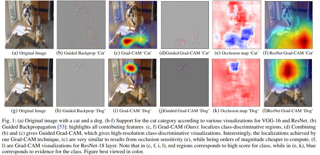
The above figure shows visualization examples from the paper. We can see that the Grad-CAM approach is very well able to detect the regions in an image that lead to high class score. The authors even combine their Grad-CAM approach with the guided back propagation method (column d). This leads to high resolution class discriminative images.

You can also find the code implementation of the paper here.

There are a lot details in the paper along with the mathematical details and methodologies used. We will not go through those in this post. They will surely be covered in future posts.

Summary and Conclusion

In this post, we saw different approaches to saliency maps in convolutional neural networks. These help in the visual understanding and explanation of the convolutional neural network. In turn, the saliency maps in convolutional neural networks lead to better know why the model is working or not working. Note that we did not dive very deep into the approaches here. We will surely do that in future posts. I hope that this post was able to give a good high level understanding of the methods for saliency maps in convolutional neural networks.

If you have any doubts, thoughts, or suggestions, then please leave them in the comment section. I will surely address them.

You can contact me using the Contact section. You can also find me on LinkedIn, and Twitter.