Chinese Number Recognition using Deep Learning and PyTorch

As deep learning developers and practitioners, we train a lot of image classification models. And most of us start by training the famous digit MNIST dataset. Similar to that, there is also another dataset consisting of Chinese Numbers. This is a very interesting alternative to the traditional MNIST dataset. Therefore, in this tutorial, we will be carrying our Chinese Number Recognition using Deep Learning and PyTorch.

What are you going to learn in this tutorial?

• First, we will know a bit about the Chinese MNIST dataset.
• Then we will train a simple neural network on the Chinese Number dataset.
  • Specifically, we will use a slightly modified version of the LeNet architecture.

Hopefully, you are interested to follow through this tutorial, even though this is a very simple one.

About the Chinese Numbers Dataset

The Chinese Numbers dataset that we will use in this tutorial is available on Kaggle. It is the Chinese MNIST dataset. The reason being, the images appear very similar to the digit MNIST dataset because of the black background and white numbers.

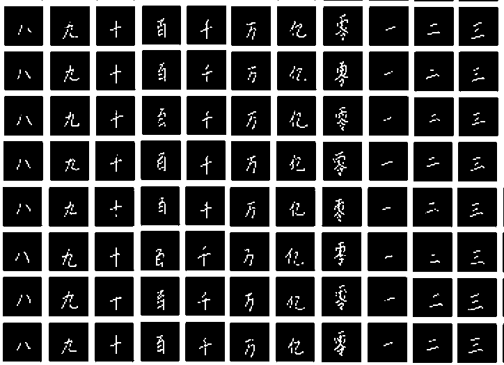
The dataset contains a total of 15 numbers. First, it contains digits from 0 to 9. In addition to that, it also contains images of digits 10, 100, 1000, 10000, and 100000000.

The following image will give you a good idea.

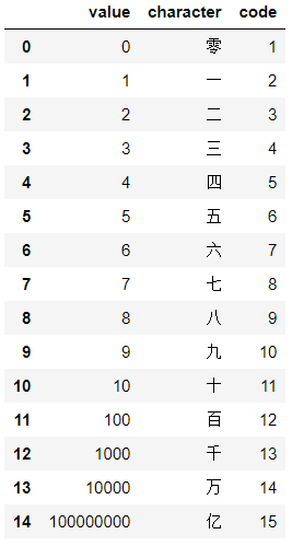
The value column contains all the numbers present in the dataset and the character contains the corresponding Chinese character/number. We can also see a code column and it is pretty important.

The code column is a mapping between the actual value of the Chinese number and a number from 1 to 15. The name of an image inside the dataset also contains this code. For example, if the name of one of the images is input_1_3_4.jpg, then the last 4 before the .jpg is the code. This means that we can very easily extract the label information while reading the image itself for training our neural network. The other two numbers are not very important for us. Still, you can visit the dataset page to know more.

One important thing to note here is that the images are of 64 x 64 x 3 dimensions. They may look like grayscale images but are actually images with three channels.

For now, go ahead and download the dataset. After extracting it, you will find all the images inside the data/data directory. Be sure to explore the images a bit. You will see two other files, namely, chinese_mnist.csv and chinese_mnist.tfrecords. We can ignore these files as we will extract the image information by reading the images and the label information from the image file name itself.

Directory Structure

Let’s take a look at the directory structure that we will be following for this project.

├── input
│   ├── chinese_mnist.csv
│   ├── chinese_mnist.tfrecords
│   └── data
│       └── data
|           ├── input_39_5_2.jpg
│           ├── input_39_5_3.jpg
│           ├── input_39_5_4.jpg
|           ...
├── outputs
│   ├── accuracy.png
│   ...
├── dataset.py
├── models.py
├── test.py
├── train.py
└── utils.py

• We have five Python files. We will get into the details of these while coding along the way.
• The input folder contains the extracted Chinese MNIST dataset. You can move your extracted dataset inside the input folder as well if you have it somewhere outside that folder. Now input/data/data should contain all the images and we can ignore the CSV and .tfrecords file.
• And the outputs folder will contain all the output files like the trained model and training plots among others after we have trained our neural network.

The PyTorch Version

The code in this post uses PyTorch version 1.8.0. A slightly lower or even the latest version (at the time of reading this) should not cause any issues as well. If you want to install/upgrade PyTorch, then please visit the official site and choose the installation command as per your requirements.

Chinese Number Recognition using Deep Learning and PyTorch

From this section, we will start with the coding part of the tutorial. We have five .py files in total and we will go through the code in detail wherever required.

Let’s start with some utility code and helper functions that will make our work easier along the way.

Writing Some Helper Functions

All the code in this section will go into the utils.py Python file.

Starting with the import statements and the label_mapper dictionary (will get into the details after the code).

import torch
import matplotlib.pyplot as plt

# dictionary to map the `code` of a digit to the actual value 
label_mapper = {
    1: 0,
    2: 1,
    3: 2,
    4: 3,
    5: 4,
    6: 5,
    7: 6,
    8: 7,
    9: 8,
    10: 9,
    11: 10,
    12: 100,
    13: 1000,
    14: 10000,
    15: 100000000
}

The label_mapper dictionary in the above code block maps the code of a Chinese number to the actual value. We discussed this while getting to know about the dataset in one of the previous sections. The last number in the image file name before the .jpg extension contains the code for the number. Those values are the keys of the dictionary and the actual value of the number is the corresponding values in the dictionary.

Helper Function to Extract the Label of a Chinese Number

Now let’s write the helper function that will extract the label code (keys of the label_mapper dictionary) and the actual value (values of the label_mapper dictionary).

def get_digit_label(image_path):
    """
    This function returns the code for a digit and the actual value
    of the digit by mapping the `label_code` using the `label_mapper`.
    """
    digit_file_name =  image_path.split('/')[-1].split('.')[0]
    label_code = int(digit_file_name.split('_')[-1])
    label = label_mapper[label_code]
    return label_code, label

The get_digit_label() function accepts one image_path as the parameter. First, we split the image_path appropriately to get the label_code. This can be any number between 1 and 15 (both inclusive) which is present as one of the keys in the label_mapper dictionary. From there, we get the label at line 29 using the obtained label_code. The value of the label can either be any digit from 0 to 9. Or it can be any of 10, 100, 1000, 10000, or 100000000.

Function to Split the Dataset into Training and Validation Set

Here, we will write a function to split the dataset into training and validation set. Let’s check out the code first.

def train_val_split(image_paths, ratio=0.15):
    """
    This functiont takes all the `image_paths` list and 
    splits the into a train and validation list.
    
    :param image_paths: list containing all the image paths
    :param ratio: train/test split ratio
    """
    num_images = len(image_paths)
    valid_ratio = int(num_images*ratio)
    train_ratio = num_images - valid_ratio
    train_images = image_paths[0:train_ratio]
    # leave the last 10 images to use them in final testing
    valid_images = image_paths[train_ratio:-10] 
    return train_images, valid_images

So, the train_val_split() function accepts the image_paths list containing the path to all the images and the split ratio as parameters. We are using 85% of the data for training and around 15% of the data for validation (but not exactly). We are leaving out the last 10 images while preparing the list for the valid_images (line 44). This is because we will use these 10 images for the final testing after we have completed the model training and validation.

The function returns the train_images and valid_images lists. The lists contain 12750 and 2240 image paths respectively.

Function to Save the Trained Model

Next, we will write a very simple function to save the trained model.

def save_model(epochs, model, optimizer, criterion):
    """
    Function to save the trained model to disk.
    """
    torch.save({
                'epoch': epochs,
                'model_state_dict': model.state_dict(),
                'optimizer_state_dict': optimizer.state_dict(),
                'loss': criterion,
                }, 'outputs/model.pth')

We are saving the model’s state_dict() along with the total number of epochs, the optimizer parameters, and the loss function. This is a very desirable and good practice rather than saving the entire model as this will allow us to continue training in the future if we want to do so.

Function to Save the Training and Validation Plots

The final helper function saves the training and validation plots for the accuracy and loss values while training.

def save_plots(train_acc, valid_acc, train_loss, valid_loss):
    """
    Function to save the loss and accuracy plots to disk.
    """
    # accuracy plots
    plt.figure(figsize=(10, 7))
    plt.plot(
        train_acc, color='green', linestyle='-', 
        label='train accuracy'
    )
    plt.plot(
        valid_acc, color='blue', linestyle='-', 
        label='validataion accuracy'
    )
    plt.xlabel('Epochs')
    plt.ylabel('Accuracy')
    plt.legend()
    plt.savefig('outputs/accuracy.png')
    plt.show()
    # loss plots
    plt.figure(figsize=(10, 7))
    plt.plot(
        train_loss, color='orange', linestyle='-', 
        label='train loss'
    )
    plt.plot(
        valid_loss, color='red', linestyle='-', 
        label='validataion loss'
    )
    plt.xlabel('Epochs')
    plt.ylabel('Loss')
    plt.legend()
    plt.savefig('outputs/loss.png')
    plt.show()

The save_plots() function accepts the lists containing the training & validation accuracy and loss values. It then saves the plots to disk in the outputs folder.

This completes all the utility function that we need.

The Neural Networks Architecture

We will use a very simple modified version of the LeNet architecture. Traditionally, the LeNet arhitecture was designed to take grayscale (single color channel) images as input. We will just modify it to accept colored images (3 channels) and keep rest of the architecture the same.

This code will go into the models.py Python file.

import torch
import torch.nn as nn
import torch.nn.functional as F

# a very simple modified version of the LeNet architecture
# modified for 3 channel (RGB input) instead of te more common...
# ... single channel input
class SimpleLeNet(nn.Module):
    def __init__(self):
        super().__init__()
        self.conv1 = nn.Conv2d(3, 6, 5)
        self.pool = nn.MaxPool2d(2, 2)
        self.conv2 = nn.Conv2d(6, 16, 5)
        self.fc1 = nn.Linear(16 * 5 * 5, 120)
        self.fc2 = nn.Linear(120, 84)
        self.fc3 = nn.Linear(84, 15)

    def forward(self, x):
        x = self.pool(F.relu(self.conv1(x)))
        x = self.pool(F.relu(self.conv2(x)))
        x = torch.flatten(x, 1)
        x = F.relu(self.fc1(x))
        x = F.relu(self.fc2(x))
        x = self.fc3(x)
        return x

Take a look at the architecture of the model. Nothing special going on here. The SimpleNet() architecture has two 2D convolutional layers followed by max-pooling layers. Then we have three fully connected layers with the last one being the output layer.

Preparing the Chinese MNIST Dataset

It’s time that we prepare the Chinese MNIST dataset in PyTorch format now. For that, we will write a ChineseMNISTDataset() class that will provide us with the images and labels.

We will write the dataset preparation code in the dataset.py file.

Let’s start with the import statements.

from torchvision import transforms as transforms
from utils import get_digit_label
from torch.utils.data import Dataset

import cv2

We will need the transforms module from torchvision to define the image transforms and augmentations. Along with that, are also importing the get_digit_label from our own utils module. And we need cv2 module for reading the images.

The following code block contains the entire ChineseMNISTDataset() class.

# the Chinse MNIST dataset
class ChineseMNISTDataset(Dataset):
    def __init__(self, image_list, is_train=True):
        self.image_list = image_list
        self.is_train = is_train
        
        # training transforms and augmentations
        if self.is_train:
            self.transform = transforms.Compose([
                transforms.ToPILImage(),
                transforms.Resize((32, 32)),
                transforms.ToTensor(),
                transforms.Normalize(
                                     mean=[0.5, 0.5, 0.5],
                                     std=[0.5, 0.5, 0.5]
                )
            ])
            
        # validation transforms
        if not self.is_train:
            self.transform = transforms.Compose([
                transforms.ToPILImage(),
                transforms.Resize((32, 32)),
                transforms.ToTensor(),
                transforms.Normalize(
                                     mean=[0.5, 0.5, 0.5],
                                     std=[0.5, 0.5, 0.5]
                )
            ])
            
    def __len__(self):
        return len(self.image_list)
    
    def __getitem__(self, index):
        image = cv2.imread(self.image_list[index])
        image = cv2.cvtColor(image, cv2.COLOR_BGR2RGB)
        image = self.transform(image)
        label_code, label = get_digit_label(self.image_list[index])
        label_code = label_code - 1
        
        return {
            'image': image,
            'label': label_code
        }

• In the __init__() method, we initialize two variables, image_list and is_train. The image_list variable contains the paths either to the training images or the validation images. And the is_train variable specifies whether the current list is for training or validation.
• We define the image transforms and augmentations according to the value of the is_train variable. Although in our case, both our transforms are the same, mostly it is not the case and the is_train variable will help in those cases. For the augmentations, we are just resizing the images to 32×32 dimensions.
• In the __getitem__() method, first, we read the image and convert it to the RGB color format. Then we apply the image transforms.
• At line 43, we get the label_code and label of the image by calling the get_digit_label() function. Please take a close look at line 44. We subtract 1 from the label_code value. This is because, currently, the label_code value is between 1 and 15. But the neural networks will want labels to start from 0. So, we subtract 1 to make the labels range from 0 to 14. Whenever we will extract the label from the predictions, first, we will have to add 1 and then map using the label_mapper dictionary.

This completes the code for preparing the dataset for Chinese MNIST images.

Writing the Training Code

This section is going to be pretty simple as most of the things are ready by now. We will write the training code in the train.py Python script.

Let’s start with the import statements.

from utils import train_val_split, save_model, save_plots
from dataset import ChineseMNISTDataset
from torch.utils.data import DataLoader
from tqdm import tqdm

import glob
import torch
import models
import torch.nn as nn
import torch.optim as optim
import matplotlib

matplotlib.style.use('ggplot')

• First, we are importing all the required functions from the utils module.
• Then the ChineseMNISTDataset class from the dataset module.
• All the others are library-specific modules that we need along the way.

Let’s define some of the training parameters as well.

# training parameters
epochs = 20
batch_size = 32
device = 'cpu'

We will train the model for 20 epochs with a batch size of 32. Also, our computation device is CPU. The dataset contains around 15000 images and the training will be fairly fast even on a CPU. If you wish to train on a GPU, just change the device value to cuda.

Datasets and Data Loaders

Now we need to prepare our training and validation dataset and dataloaders. The following block contains the code for that.

# capture all the image paths
image_paths = glob.glob('input/data/data/*.jpg')

# get the train and validation image paths lists
train_images, valid_images = train_val_split(image_paths)
print(f"Number of training images: {len(train_images)}")
print(f"Numher of test images: {len(valid_images)}")
# training and validation dataset
train_dataset = ChineseMNISTDataset(train_images, is_train=True)
valid_dataset = ChineseMNISTDataset(valid_images, is_train=False)
# training and validation data loader
train_dataloader = DataLoader(train_dataset, batch_size=batch_size, shuffle=True)
valid_dataloader = DataLoader(valid_dataset, batch_size=batch_size, shuffle=False)

• The image_paths list contains the paths to all the images.
• At line 22, we split the above image_paths list into a train_images list and valid_images list.
• Lines 26 and 27 provide the train_dataset and valid_dataset by initializing the ChineseMNISTDataset() class.
• At lines 29 and 30, we prepare the train_dataloader and valid_dataloader.

Now, let’s initialize the model, the loss function and the optimizer.

# initialize the model
model = models.SimpleLeNet()
# the loss function
criterion = nn.CrossEntropyLoss()
# the optimizer
optimizer = optim.Adam(model.parameters(), lr=0.001)

We are using the Cross Entropy Loss as this is a multi class problem. The optimizer is the Adam optimizer with a learning rate of 0.001.

The Training Function

The training function is going to be very similar to any other classification training function in PyTorch. The following code block defines the function.

# training
def train(model, trainloader, optimizer, criterion):
    model.train()
    print('Training')
    train_running_loss = 0.0
    train_running_correct = 0
    counter = 0
    for i, data in tqdm(enumerate(trainloader), total=len(trainloader)):
        counter += 1
        image, labels = data['image'], data['label']
        image = image.to(device)
        labels = labels.to(device)
        optimizer.zero_grad()
        # forward pass
        outputs = model(image)
        # calculate the loss
        loss = criterion(outputs, labels)
        train_running_loss += loss.item()
        # calculate the accuracy
        _, preds = torch.max(outputs.data, 1)
        train_running_correct += (preds == labels).sum().item()
        # backpropagation
        loss.backward()
        # update the optimizer parameters
        optimizer.step()
    
    # loss and accuracy for the complete epoch
    epoch_loss = train_running_loss / counter
    epoch_acc = 100. * (train_running_correct / len(trainloader.dataset))
    return epoch_loss, epoch_acc

The function is quite self-explanatory. After the completion of one epoch, we are returning the epoch-wise loss and accuracy values.

The Validation Function

In the validation function, we do not need to backpropagate the gradients. or update the optimizer parameters. Also, we are switching the model to eval() mode and the entire validation loop is inside the with torch.no_grad() block to prevent the accumulation of gradients in the memory.

# validation
def validate(model, testloader, criterion):
    model.eval()
    print('Validation')
    valid_running_loss = 0.0
    valid_running_correct = 0
    counter = 0
    with torch.no_grad():
        for i, data in tqdm(enumerate(testloader), total=len(testloader)):
            counter += 1
            
            image, labels = data['image'], data['label']
            image = image.to(device)
            labels = labels.to(device)
            # forward pass
            outputs = model(image)
            # calculate the loss
            loss = criterion(outputs, labels)
            valid_running_loss += loss.item()
            # calculate the accuracy
            _, preds = torch.max(outputs.data, 1)
            valid_running_correct += (preds == labels).sum().item()
        
    # loss and accuracy for the complete epoch
    epoch_loss = valid_running_loss / counter
    epoch_acc = 100. * (valid_running_correct / len(testloader.dataset))
    return epoch_loss, epoch_acc

Running the Training Loop

The final part is running the training loop for the desired number of epochs what we want to train for.

# lists to keep track of losses and accuracies
train_loss, valid_loss = [], []
train_acc, valid_acc = [], []
# start the training
for epoch in range(epochs):
    print(f"[INFO]: Epoch {epoch+1} of {epochs}")
    train_epoch_loss, train_epoch_acc = train(model, train_dataloader, 
                                              optimizer, criterion)
    valid_epoch_loss, valid_epoch_acc = validate(model, valid_dataloader,  
                                                 criterion)
    train_loss.append(train_epoch_loss)
    valid_loss.append(valid_epoch_loss)
    train_acc.append(train_epoch_acc)
    valid_acc.append(valid_epoch_acc)
    print(f"Training loss: {train_epoch_loss:.3f}, training acc: {train_epoch_acc:.3f}")
    print(f"Validation loss: {valid_epoch_loss:.3f}, validation acc: {valid_epoch_acc:.3f}")
    print('-'*50)

# save the trained model weights
save_model(epochs, model, optimizer, criterion)
# save the loss and accuracy plots
save_plots(train_acc, valid_acc, train_loss, valid_loss)

print('TRAINING COMPLETE')

• First, we define four lists to store the per-epoch validation and training loss as well as accuracy values.
• While looping through the epochs, we append each epochs’s loss and accuracy values to the respective lists and print the current epochs’s loss and accuracy as well.

After the training completes, we save the model checkpoint at line 113. We also save the loss and accuracy plots at line 115.

This completes our entire training script. Now, we are ready to execute train.py and start the training.

Executing train.py to for Chinese Number Recognition using Deep Learning

Now it’s time to train our simple and modified “LeNet” model on the Chinese MNIST dataset.

Go into the project directory and open up the terminal/command line. Then type the following command.

python train.py

You should see output similar to the following on the terminal.

Number of training images: 12750
Numher of test images: 2240
[INFO]: Epoch 1 of 20
Training
100%|█████████████████████████████████████████| 399/399 [00:40<00:00,  9.88it/s]
Validation
100%|███████████████████████████████████████████| 70/70 [00:06<00:00, 10.58it/s]
Training loss: 2.185, training acc: 27.843
Validation loss: 1.485, validation acc: 51.652
--------------------------------------------------
[INFO]: Epoch 2 of 20
Training
100%|█████████████████████████████████████████| 399/399 [00:04<00:00, 80.00it/s]
Validation
100%|███████████████████████████████████████████| 70/70 [00:00<00:00, 95.15it/s]
Training loss: 1.220, training acc: 59.224
Validation loss: 1.041, validation acc: 63.839
--------------------------------------------------
...
[INFO]: Epoch 20 of 20
Training
100%|█████████████████████████████████████████| 399/399 [00:05<00:00, 73.09it/s]
Validation
100%|███████████████████████████████████████████| 70/70 [00:00<00:00, 84.38it/s]
Training loss: 0.158, training acc: 94.416
Validation loss: 0.227, validation acc: 92.902
--------------------------------------------------
TRAINING COMPLETE

The training should only take a few minutes even on a CPU. After the training completes, you should see the accuracy and loss graphs in the outputs folder along with the saved checkpoint, model.pth.

Analyzing the Outputs

By the end of training, we can see that the training loss and accuracy are 0.158 and 94.416% respectively. And the validation loss and accuracy are 0.227 and 92.902% respectively. Not bad considering we used such a simple model and the Chinese characters were not that easy to recognize as well.

How about the graphs that are saved to the disk?

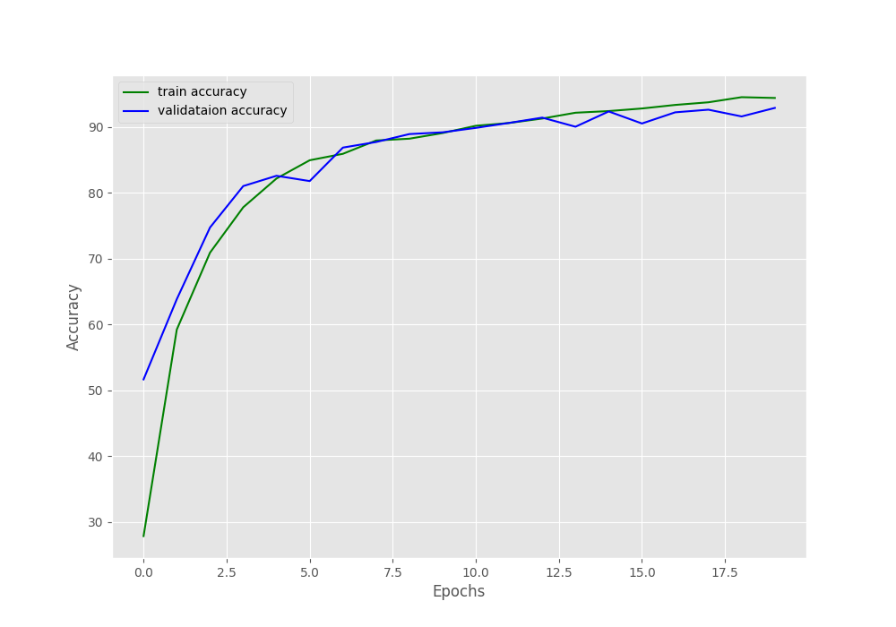
From the curve, the model seems to be learning well. By the end of the training, the validation accuracy values are lower than the training accuracy values.

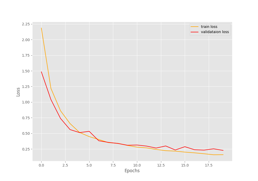
The loss curves seems quite good as well. Both validation and training loss values were decreasing till the end.

From the graphs it appears that training for a few more epochs would could have given even better results.

Testing the Trained Model on Unseen Chinese Numbers

Now, that we know how the model performs during training, how about testing the model on unseen images.

Remember we had left out 10 images from the validation set so that we can test the model later on. Let’s write a simple script for that. It will be fun to see how well the model performs on unseen images.

All of this code will go into the test.py script.

As usual, starting with the imports.

import torch
import cv2
import glob as glob
import torchvision.transforms as transforms
import numpy as np

from models import SimpleLeNet
from utils import label_mapper, get_digit_label

Next, define the computation device, load the model checkpoint and the trained weights, and define the image transforms.

# inferencing on CPU
device = 'cpu'
# initialize the model
model = SimpleLeNet()
# load the model checkpoint
checkpoint = torch.load('outputs/model.pth')
# load the trained weights
model.load_state_dict(checkpoint['model_state_dict'])
model.to(device)
model.eval()
# simple image transforms
transform = transforms.Compose([
    transforms.ToPILImage(),
    transforms.Resize((32, 32)),
    transforms.ToTensor(),
    transforms.Normalize(
                         mean=[0.5, 0.5, 0.5],
                         std=[0.5, 0.5, 0.5]
    )
])

We are loading the checkpoint at line 14. After that the trained weights are being loaded at line 16. Then we are switching the model to eval() mode and loading it onto the computation device. The image transforms are same as we had for validation.

We will read the last 10 images from the image directory and iterate over one image at a time while predicting the value for it.

# get the paths for the last ten images
image_paths = glob.glob('input/data/data/*.jpg')[-10:]
for i, image_path in enumerate(image_paths):
    label_code, actual_label = get_digit_label(image_path)
    orig_img = cv2.imread(image_path)
    # convert to from BGR to RGB color
    image = cv2.cvtColor(orig_img, cv2.COLOR_BGR2RGB)
    image = transform(image)
    # add one extra batch dimension
    image = image.unsqueeze(0).to(device)
    # forward pass the image through the model
    outputs = model(image)
    # get the index of the highest score
    label = np.array(outputs.detach()).argmax()
    predicted_label = label_mapper[label+1]
    print(f"GT: {actual_label}, Pred: {predicted_label}")
    # put the actual label on the original image
    cv2.putText(orig_img, f"g:{actual_label}", (1, 10), cv2.FONT_HERSHEY_SIMPLEX, 
                0.3, (0, 255, 0), 1)
    # put the predicted label on the original image
    cv2.putText(orig_img, f"p:{predicted_label}", (1, 20), cv2.FONT_HERSHEY_SIMPLEX, 
                0.3, (0, 255, 0), 1)

    # resize the final result
    orig_img = cv2.resize(orig_img, (224, 224))
    # show and save the resutls
    cv2.imshow('Result', orig_img)
    cv2.waitKey(100)
    cv2.imwrite(f"outputs/result_{i}.jpg", orig_img)

• At line 30, we are obtaining the paths for the last 10 images and keeping them in the image_paths list.
• Then we start to iterate over each of the image paths. At line 32, we get the label_code and the actual_label of the Chinese number.
• The next few lines read the image, change the color format, apply the transforms, and add an extra batch dimension.
• We forward pass the image through the model at line 40 and get the predicted label at line 42.
• Remember we have to add 1 to the predicted label before mapping it to the actual number using the label_mapper. This, we are doing at line 43.
• We are also showing the ground truth and predicted value on the terminal.
• Lines 46 and 49 put the ground truth text and predicted label text on the image.
• The final few lines enlarges the image for proper visualization, shows the image on screen, and saves the output to disk.

This completes the test script as well. Now, let’s run it and see what king of results we get.

Execute test.py to Test on Unseen Images

Just execute the following command on the terminal while being within the project directory.

python test.py

You should the following output on the terminal.

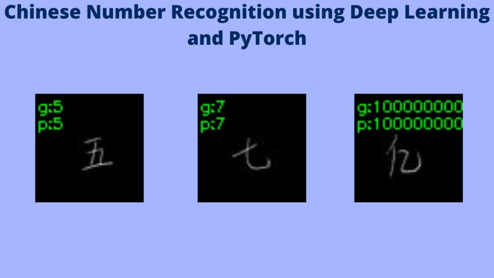
GT: 5, Pred: 5
GT: 10, Pred: 1000
GT: 10, Pred: 10
GT: 7, Pred: 7
GT: 5, Pred: 5
GT: 100000000, Pred: 100000000
GT: 1000, Pred: 1000
GT: 10000, Pred: 10000
GT: 5, Pred: 5
GT: 10000, Pred: 1000

You can see that the model predicted two of the number of incorrectly. It predicted one of the numbers as 1000 instead of 10 and again one as 1000 instead of 10000.

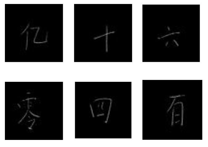
Although, we cannot visualize all the 10 images that are saved to disk, the following figure shows some of the results along with the incorrect ones.

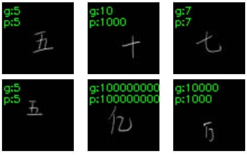
Figure 6 shows six out of 10 output images. This also includes the 2 wrong predictions that we discussed just above. Considering such a simple model, overall, the results are quite good. Using a slightly more complex model and training for a few more epochs should give even better results.

If you try something new, then do share your results in the comment section. This will also help and inspire others.

Want to Get Started with PyTorch?

If you are new to PyTorch and want to get started with it, then please visit the Deep Learning with Pytorch series.

Deep Learning with PyTorch: Image Classification using Neural Networks

Summary and Conclusion

In this tutorial, you learned about Chinese Number Recognition using Deep Learning and PyTorch. We used a very simple model to train on the Chinese MNIST data which performed pretty well. Obviously, some more tweaks will improve the results. I hope that you learned something new from this tutorial.

If you have any doubts, thoughts, or suggestions, then please leave them in the comment section. I will surely address them.

You can contact me using the Contact section. You can also find me on LinkedIn, and Twitter.