Deep Learning with PyTorch: Image Classification using Neural Networks

In this tutorial, we are going to learn how to carry out image classification using neural networks in PyTorch. Basically, we will build convolutional neural network models for image classification.

This is the fourth part of the series, Deep Learning with PyTorch.
Part 1: Installing PyTorch and Covering the Basics.
Part 2: Basics of Autograd in PyTorch.
Part 3: Basics of Neural Network in PyTorch.
Part 4: Image Classification using Neural Networks.

What will we be covering in this article?

• We will start off with classifying the all famous Digit MNIST dataset.
• With Digit MNIST, we will see a very simple neural network with PyTorch and keep track of the loss while training.
• Then we will move on to Fashion MNIST which we will classify using the LeNet architecture.
• For Fashion MNIST, we will calculate the training and testing accuracy along with the loss values.
• We will also visualize the results using graphical plots.

If you are following my article, then you must remember that we got to know the basics of neural network construction in the previous article. We used the LeNet architecture for that. In this article, for the Digit MNIST dataset, we will use a smaller network. And for the Fashion MNIST classification, we will use the LeNet architecture. If you are new to this series, then I highly suggest that you go through the previous article. In that way, we can concentrate on the concepts that are most important.

Let’s start with the classification of Digit MNIST images.

Digit MNIST Classification using PyTorch

First, we need to import all the libraries and modules that we will need further on.

import torch
import torchvision
import torchvision.transforms as transforms
import torch.nn as nn
import torch.nn.functional as F
import torch.optim as optim
import numpy as np
import matplotlib.pyplot as plt
import time

from torchvision import datasets

• torchvision is one of the most important modules of PyTorch. We can download many datasets using torchvision. For this one, we will need the Digit MNIST dataset and we will download that.
• torchvision.transforms will help us in the transformation of the pixel value of the images. Mainly what we call as normalization and standardization.

Now, let’s define the transforms that we want to apply to the dataset.

Defining the Transforms

transform = transforms.Compose(
    [transforms.ToTensor(),
     transforms.Normalize((0.5,), (0.5,))]
)

First of all, we convert the dataset to tensors. This is the heart of PyTorch as all operations happen on tensors only. Next, we normalize the dataset. Now, what does Normalize((0.5,), (0.5,)) mean. Remember that all the images are grayscale. Therefore, the channel is one. The 0.5 defines the mean and standard deviation for each channel. So, basically the concept is, Normalize((mean_channel1, ), (std_channel1)). Had it been three channels (RGB), then it would have been Normalize((0.5, 0.5, 0.5), (0.5, 0.5, 0.5)). I hope that you are clear on this concept.

Download the Data

To download the dataset, we can use torchvision.datasets.

# get the data
trainset = datasets.MNIST(
    root = './data',
    train = True,
    download = True, 
    transform = transform
)

trainloader = torch.utils.data.DataLoader(
    trainset, 
    batch_size = 4,
    shuffle = True
)

testset = datasets.MNIST(
    root = './data',
    train = False,
    download = True,
    transform = transform
)

testloader = torch.utils.data.DataLoader(
    testset, 
    batch_size = 4,
    shuffle = False
)

You can see that in datasets.MNIST(), one of the arguments is transform=transform. This will directly transform the data into tensors and normalize the pixels as well.

Also, you can observe that we have trainloader and testloader. Both of them have batch_size as 4. The MNIST dataset has 60000 training instances. With this batch size, we will have 15000 batches in total for trainloader. Using torch.utils.data.DataLoader to convert the data into batches will greatly help us in the later stages.

Visualize the Images

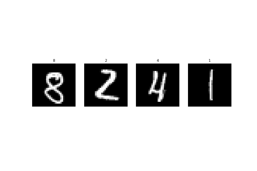
Next, to visualize the images, we can take the first batch. This will contain 4 images.

for batch_1 in trainloader:
    batch = batch_1
    break

print(batch[0].shape) # as batch[0] contains the image pixels -> tensors
print(batch[1]) # batch[1] contains the labels -> tensors

plt.figure(figsize=(12, 8))
for i in range (batch[0].shape[0]):
    plt.subplot(1, 4, i+1)
    plt.axis('off')
    plt.imshow(batch[0][i].reshape(28, 28), cmap='gray')
    plt.title(int(batch[1][i]))
    plt.savefig('digit_mnist.png')
plt.show()

Define the Neural Network

Here, we will define our neural network module and call it Net().

class Net(nn.Module):
    def __init__(self):
        super(Net, self).__init__()
        self.conv1 = nn.Conv2d(in_channels=1, out_channels=20, 
                               kernel_size=5, stride=1)
        self.conv2 = nn.Conv2d(in_channels=20, out_channels=50, 
                               kernel_size=5, stride=1)
        self.fc1 = nn.Linear(in_features=800, out_features=500)
        self.fc2 = nn.Linear(in_features=500, out_features=10)

    def forward(self, x):
        x = F.relu(self.conv1(x))
        x = F.max_pool2d(x, 2, 2)
        x = F.relu(self.conv2(x))
        x = F.max_pool2d(x, 2, 2)
        x = x.view(x.size(0), -1)
        x = F.relu(self.fc1(x))
        x = self.fc2(x)
        return x

This is a very small network but it is enough for Digit MNIST dataset. Often while training deep neural networks, it is better to have an Nvidia GPU available. PyTorch provides really easy functionality to use GPU if available. The following line of code does the trick.

device = torch.device('cuda:0' if torch.cuda.is_available() else 'cpu')

Now, if you have a GPU, then it will be selected, else the CPU will be selected for further calculations. Although this problem does not specifically require a GPU, it is always better to have a CUDA device for faster training and testing of deep neural networks.

We can instantiate our Net() module and also transfer it onto the device. If you have a CUDA, then it will be transferred to the CUDA device.

net = Net().to(device)
print(net)

Net(
  (conv1): Conv2d(1, 20, kernel_size=(5, 5), stride=(1, 1))
  (conv2): Conv2d(20, 50, kernel_size=(5, 5), stride=(1, 1))
  (fc1): Linear(in_features=800, out_features=500, bias=True)
  (fc2): Linear(in_features=500, out_features=10, bias=True)
)

Optimizer and Loss Function

In this section, we will define the optimizer and loss function for our neural network. We will be using CrossEntropyLoss and SGD() as the loss function and optimizer respectively.

# loss function
criterion = nn.CrossEntropyLoss()
# optimizer
optimizer = optim.SGD(net.parameters(), lr=0.001, momentum=0.9)

Training Our Neural Network on the Data

We are all set to train our neural network on the dataset. We will train for 10 epochs. Remember that we have 15000 batches with 4 images in each batch. Let’s first train our network, and then discuss the essential parts.

def train(net):
    start = time.time()
    for epoch in range(10): # no. of epochs
        running_loss = 0.0
        for i, data in enumerate(trainloader, 0):
            # data pixels and labels to GPU if available
            inputs, labels = data[0].to(device, non_blocking=True), data[1].to(device, non_blocking=True)
            # set the parameter gradients to zero
            optimizer.zero_grad()
            outputs = net(inputs)
            loss = criterion(outputs, labels)
            # propagate the loss backward
            loss.backward()
            optimizer.step()

            # print for mini batches
            running_loss += loss.item()
            if i % 5000 == 4999:  # every 5000 mini batches
                print('[Epoch %d, %5d Mini Batches] loss: %.3f' %
                      (epoch + 1, i + 1, running_loss/5000))
                running_loss = 0.0
    end = time.time()

    print('Done Training')
    print('%0.2f minutes' %((end - start) / 60))
    
train(net)

[Epoch 1,  5000 Mini Batches] loss: 0.298
[Epoch 1, 10000 Mini Batches] loss: 0.084
[Epoch 1, 15000 Mini Batches] loss: 0.061
[Epoch 2,  5000 Mini Batches] loss: 0.044
[Epoch 2, 10000 Mini Batches] loss: 0.040
[Epoch 2, 15000 Mini Batches] loss: 0.039
...
[Epoch 10,  5000 Mini Batches] loss: 0.003
[Epoch 10, 10000 Mini Batches] loss: 0.005
[Epoch 10, 15000 Mini Batches] loss: 0.005
Done Training
15.91 minutes

So, in the above code block, we are printing the loss every 5000 mini-batches. This helps to keep track of whether our network is really learning or not. For this specific problem, our network seems to be learning well. We have a loss of 0.005 by the end of training which is good for a start. Also, note that at line 7, we are transferring the pixels data and the corresponding labels to the device. Now, this can be either the CPU or the GPU depending on the system. The important thing to remember here is that we need to do it for every epoch and batch.

Testing Our Network on the Test Set

Okay, it’s time to see how our model performs on the unseen test data. You must be remembering how we need to backpropagate our gradients while training so that our model can learn. Well, we do not need to do that during testing.

Therefore, our testing phase will look very similar to the training phase, but we will not calculate the gradients and everything will run within the torch.no_grad() block, so that the gradients do not get calculated. This might sound confusing, but it will become very clear after you see the code once.

correct = 0
total = 0
with torch.no_grad():
    for data in testloader:
        inputs, labels = data[0].to(device, non_blocking=True), data[1].to(device, non_blocking=True)
        outputs = net(inputs)
        _, predicted = torch.max(outputs.data, 1)
        total += labels.size(0)
        correct += (predicted == labels).sum().item()

print('Accuracy of the network on test images: %0.3f %%' % (
    100 * correct / total))

Accuracy of the network on test images: 99.210 %

We are getting an accuracy of 99.21 % which is good for a start. If you want to further increase your knowledge, then you should try to achieve even better accuracy by tweaking the above code. Trying that will help you understand many of the underlying concepts as well.

Next, we will classify Fashion MNIST images using PyTorch as well.

Fashion MNIST Classification using PyTorch

In this section, we will classify the Fashion MNIST images using PyTorch. We will use LeNet CNN architecture to classify the images.

In the previous section, with the MNIST digits, we just evaluated the loss. But here, we will evaluate the loss, the training accuracy, and the testing accuracy as well. Along with that, we will also take a look at the plots of all those evaluations for better clarifications.

The first few parts are going to be the same as the Digit MNIST section, where we import the modules, download the dataset, and visualize the images.

Imports

import torch
import matplotlib.pyplot as plt
import numpy as np
import torchvision
import torchvision.transforms as transforms
import torch.nn as nn
import torch.nn.functional as F
import torch.optim as optim
import time

Defining some constants

We are defining some constants here, that will make our work easier to manage the code.

# define constants
NUM_EPOCHS = 10
BATCH_SIZE = 4
LEARNING_RATE = 0.001

Defining the transforms

transform = transforms.Compose(
    [transforms.ToTensor(),
     transforms.Normalize((0.5,), (0.5,))])

Download the Data

trainset = torchvision.datasets.FashionMNIST(root='./data', train=True,
                                             download=True, 
                                             transform=transform)
testset = torchvision.datasets.FashionMNIST(root='./data', train=False,
                                            download=True, 
                                            transform=transform)

trainloader = torch.utils.data.DataLoader(trainset, batch_size=BATCH_SIZE,
                                          shuffle=True)
testloader = torch.utils.data.DataLoader(testset, batch_size=BATCH_SIZE,
                                          shuffle=True)

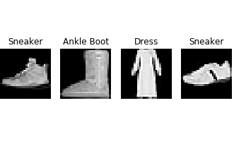
Visualize the images

To visualize the images along with labels, we will need the names of the fashion items. You can get that from the official GitHub repository.

classes = ('T-Shirt','Trouser','Pullover','Dress','Coat','Sandal',
           'Shirt','Sneaker','Bag','Ankle Boot')

Now, let’s visualize the images.

for batch_1 in trainloader:
    batch = batch_1
    break

print(batch[0].shape) # as batch[0] contains the image pixels -> tensors
print(batch[1].shape) # batch[1] contains the labels -> tensors

plt.figure(figsize=(12, 8))
for i in range (batch[0].shape[0]):
    plt.subplot(4, 8, i+1)
    plt.axis('off')
    plt.imshow(batch[0][i].reshape(28, 28), cmap='gray')
    plt.title(classes[batch[1][i]])
    plt.savefig('fashion_mnist.png')
plt.show()

Build LeNet CNN Architecture

Here, we will define a module to build the LeNet CNN architecture. We will use the nn.Module from PyTorch to define all the layers. The following is the code defining the LeNet() class.

class LeNet(nn.Module):
    def __init__(self):
        super(LeNet, self).__init__()
        self.conv1 = nn.Conv2d(in_channels=1, out_channels=6, 
                               kernel_size=5)
        self.conv2 = nn.Conv2d(in_channels=6, out_channels=16, 
                               kernel_size=5)
        self.fc1 = nn.Linear(in_features=256, out_features=120)
        self.fc2 = nn.Linear(in_features=120, out_features=84)
        self.fc3 = nn.Linear(in_features=84, out_features=10)
        
    def forward(self, x):
        x = F.relu(self.conv1(x))
        x = F.max_pool2d(x, kernel_size=2)
        x = F.relu(self.conv2(x))
        x = F.max_pool2d(x, kernel_size=2)
        x = x.view(x.size(0), -1)
        x = F.relu(self.fc1(x))
        x = F.relu(self.fc2(x))
        x = self.fc3(x)
        return x

net = LeNet()
print(net)

LeNet(
  (conv1): Conv2d(1, 6, kernel_size=(5, 5), stride=(1, 1))
  (conv2): Conv2d(6, 16, kernel_size=(5, 5), stride=(1, 1))
  (fc1): Linear(in_features=256, out_features=120, bias=True)
  (fc2): Linear(in_features=120, out_features=84, bias=True)
  (fc3): Linear(in_features=84, out_features=10, bias=True)
)

Loss Function and Optimizer

We will use the CrossEntropyLoss and SGD optimizer this time as well

# loss function and optimizer
loss_function = nn.CrossEntropyLoss()
optimizer = optim.SGD(net.parameters(), lr=LEARNING_RATE, momentum=0.9)

Training

We are all set to train our neural network. But before that, let’s define our device where the training will take place. This is will choose the CUDA device, if available, else the training will take place on the CPU. Also, we will transfer our network onto the device.

# if GPU is available, then use GPU, else use CPU
device = torch.device('cuda:0' if torch.cuda.is_available() else 'cpu')
print(device)
net.to(device)

The next function that we are defining is a simple yet important one. That will help us to calculate the training accuracy on the training data and the validation accuracy on the test data.

# function to calculate accuracy
def calc_acc(loader):
    correct = 0
    total = 0
    for data in loader:
        inputs, labels = data[0].to(device), data[1].to(device)
        outputs = net(inputs)
        _, predicted = torch.max(outputs.data, 1)
        total += labels.size(0)
        correct += (predicted == labels).sum().item()
        
    return ((100*correct)/total)

Next is the function to train our network. Take a moment and analyze what is happening inside the function.

def train():
    epoch_loss = []
    train_acc = []
    test_acc = []
    for epoch in range(NUM_EPOCHS):
        running_loss = 0
        for i, data in enumerate(trainloader, 0):
            inputs, labels = data[0].to(device), data[1].to(device)

            # set parameter gradients to zero
            optimizer.zero_grad()

            # forward pass
            outputs = net(inputs)
            loss = loss_function(outputs, labels)
            loss.backward()
            optimizer.step()

            running_loss += loss.item()

        epoch_loss.append(running_loss/15000)
        train_acc.append(calc_acc(trainloader))
        test_acc.append(calc_acc(testloader))
        print('Epoch: %d of %d, Train Acc: %0.3f, Test Acc: %0.3f, Loss: %0.3f'
              % (epoch+1, NUM_EPOCHS, train_acc[epoch], test_acc[epoch], running_loss/15000))
        
    return epoch_loss, train_acc, test_acc

This is a very similar function that we have used for Digit MNIST classification with some minor changes.

First, we have three lists, namely, epoch_loss, train_acc, test_acc. These three store loss, training accuracy, and testing accuracy for each of the 10 epochs. We also return these three finally. Along with that, we are printing the losses and accuracies at the end of each epoch.

We are ready to train our network and see how it performs.

start = time.time()
epoch_loss, train_acc, test_acc = train()
end = time.time()

print('%0.2f minutes' %((end - start) / 60))

Epoch: 1 of 10, Train Acc: 85.010, Test Acc: 84.390, Loss: 0.638
Epoch: 2 of 10, Train Acc: 87.400, Test Acc: 86.180, Loss: 0.370
...
Epoch: 9 of 10, Train Acc: 91.867, Test Acc: 89.220, Loss: 0.226
Epoch: 10 of 10, Train Acc: 91.943, Test Acc: 88.920, Loss: 0.217

By the end of the training, we are getting about 89 % test accuracy.

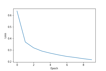
By visualizing the loss and accuracy plots we can get a better analyze the procedure.

Visualizing the Line Graphs

plt.figure()
plt.plot(epoch_loss)
plt.xlabel('Epoch')
plt.ylabel('Loss')
plt.savefig('fashion_loss.png')
plt.show()

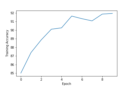
plt.figure()
plt.plot(train_acc)
plt.xlabel('Epoch')
plt.ylabel('Training Accuracy')
plt.savefig('fashion_train_acc.png')
plt.show()

plt.figure()
plt.plot(test_acc)
plt.xlabel('Epoch')
plt.ylabel('Test Accuracy')
plt.savefig('fashion_test_acc.png')
plt.show()

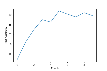
The loss is around 0.217 by the end of 10 epochs. Surely, it is not state of the art result, but it is not bad for such a simple network also. The training accuracy is above 92 % and the test accuracy is around 89 %. A bigger network will surely help in getting better results.

Before You Go…

Before you go ahead to train your own neural network with PyTorch, you may want to take a look at this amazing post. In this article, Machine Learning Number Recognition – From Zero to Application, you will learn how to build a complete web app for handwritten digit recognizer. After going through the post, you will have complete knowledge on how to build an actual deep learning based web app.

Summary and Conclusion

I hope that you learned new things about PyTorch from this article and are equipped with enough knowledge of PyTorch now that you can try new things on other datasets as well. Leave your thoughts in the comment section and I will try my best to address them.

If you like this website, do consider subscribing so as not miss any updates. You can find me on LinkedIn and Twitter as well.