Deep Learning with PyTorch: Basics of Neural Network in PyTorch

In this article, we will get to learn the basics of neural networks and how to build them using PyTorch. Essentially we will use the torch.nn package and write Python class to build a neural network in PyTorch. This is one of the most flexible and best methods to do so.

This is the third part of the series, Deep Learning with PyTorch.
Part 1: Installing PyTorch and Covering the Basics.
Part 2: Basics of Autograd in PyTorch.
Part 3: Basics of Neural Network in PyTorch.

If you are new to the series, consider visiting the previous article. They cover the basics of tensors and autograd package in PyTorch. Still, if you are comfortable enough, then you can carry on with this article directly.

What will we cover in this article?

• Knowing the torch.nn package in PyTorch.
• Building a simple neural network architecture.
• Defining optimizers, and loss functions in PyTorch.
• How to backpropagate the gradients?

We will be using the famous LeNet-5 architecture in this article.

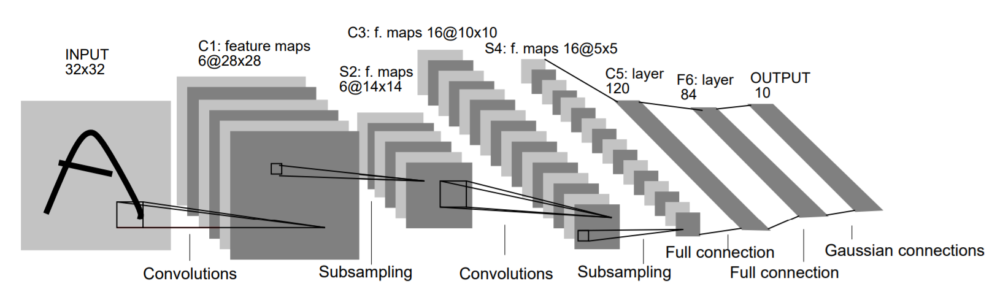
This is the same architecture that is covered in the official PyTorch tutorials. I will try to make this article as detailed and easy to follow as possible. You can always put down your queries in the comment section and I will try my best to answer them.

The torch.nn Package

We will use the torch.nn package from PyTorch to construct neural networks. We also have the class, torch.nn.Module which is the base class for all neural network modules.

Basically, nn.Module contains all the neural network layers you can think of, like convolutional, and linear layers.

Then we have the torch.nn.Functional package. This will help us to define all the intermediate operations during the forward pass of the network. Pooling operations, assigning the dropout and activation functions include some of those.

Defining Our Neural Network

Let’s start by importing the three above mentioned packages. Then we can get down to defining our network architecture.

import torch
import torch.nn as nn
import torch.nn.functional as F

Now, we will write a class using Python that will use the torch.nn.Module to construct our neural network.

We will get to the explanation part and how everything works after we write the code. That way it will be a lot easier to understand everything. Remember that we are trying to construct the Lenet-5 architecture. The following is the code for our neural network using PyTorch.

class Net(nn.Module):

    def __init__(self):
        super(Net, self).__init__()
        self.conv1 = nn.Conv2d(1, 6, (3, 3)) # (input image channel, output channels, kernel size)
        self.conv2 = nn.Conv2d(6, 16, (3, 3))
        # in linear layer (output channels from conv2d x width x height)
        self.fc1 = nn.Linear(16 * 6 * 6, 120) # (in_features, out_features)
        self.fc2 = nn.Linear(120, 84)
        self.fc3 = nn.Linear(84, 10)

    def forward(self, x):
        x = F.max_pool2d(F.relu(self.conv1(x)), (2, 2))
        x = F.max_pool2d(F.relu(self.conv2(x)), (2, 2))
        x = x.view(x.size(0), -1)
        x = F.relu(self.fc1(x))
        x = F.relu(self.fc2(x))
        x = self.fc3(x)
        return x

model = Net()
print(model)

Net(
  (conv1): Conv2d(1, 6, kernel_size=(3, 3), stride=(1, 1))
  (conv2): Conv2d(6, 16, kernel_size=(3, 3), stride=(1, 1))
  (fc1): Linear(in_features=576, out_features=120, bias=True)
  (fc2): Linear(in_features=120, out_features=84, bias=True)
  (fc3): Linear(in_features=84, out_features=10, bias=True)
)

At first, the code may seem a bit different if you are just starting with PyTorch. But eventually, all the code and concepts will become very intuitive. So, let’s get down to the explanation of the code.

At the very beginning, we construct a Net class which inherits all the properties of nn.Module. Then we have two very important functions inside the class, they are __init__(), and forward().

In line 4, inside the __init__() function, we first call super(). This ensures that we inherit all the properties if nn.Module. Now, we can use all the methods and layers that are defined in nn.Module.

Starting from line 5, we begin to construct our neural network. First, we have Conv2d(1, 6, (3, 3)) which is a convolutional layer. The first argument inside Conv2d() is 1 which is the input image channel. If we have a given 1, then the input image must be grayscale having only one channel. If the input image will be a color image, then we have to pass 3 as the argument referring to the three color channels, red, green, and blue (RGB). The second argument is 6 which refers to the output channels of the Conv2d(). The final argument is the kernel window size, which is (3×3) square kernel window in our case.

At line 6, we have another Conv2d(). Here, the input channel is 6 which is the output from the previous convolution layer. The output channel is 16, and the kernel size is again (3×3).

Note: Please note that we are only defining the layers in the __init__(). All the operations will be carried out in the forward pass of the network, that is in the forward() function.

We can move on to the linear layer (nn.Linear()). nn.Linear() has the argument format, (in_features, out_features). Many of the newcomers to PyTorch get confused as to how the in_features are calculated. You need not worry about it, I will break it down for you step by step.

At line 8, we have nn.Linear(16*6*6, 120). Here, 16 is the output channel value from the previous convolution layer. But what about the 6*6?. Ok, suppose that our input image dimensions are 32×32 (height x width). When we give this input to the first Conv2d(), the output height and output width are calculated using the following formula.

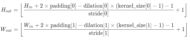
where \(H_{in}=input \ height\) (let it be 32), \(W_{in}=input \ width\) (let it be 32), \(H_{out}=output \ height\), \(W_{out}=output \ width\). And by default, \(padding\) is zero, \(dilaton\) is 1, \(stride\) is 1. Note that we have not given any values for padding, dilation, and stride, so the default values will be used.

So, using the above formula, after the first Covn2d() layer, the \(H_{out}=output \ height\) and \(W_{out}=output \ width\) are 30 and 30 respectively. Then they reduce to half, that is, 15 and 15 respectively, due to the 2×2 max-pooling in the forward pass (line 13). Similarly, after the second Conv2d() layer, the height and width become 13 and 13 respectively. Then the second 2×2 max-pooling layer reduces those to 6 and 6 respectively (line 14). And that is how we get out 16x6x6 for the in_features for our first linear layer. Finally, according to the LeNet-5 architecture we have given the out_features as 120. This covers our first linear layer at line 8 of the code.

Similarly, we have another two nn.Linear() defined. They are nn.Linear(120, 84) at line 9 and nn.Linear(84, 10) at line 10.

Now, coming to the forward() function, this is where all the operations on the layers that we have defined in __init__() takes place. We have already analyzed how max-pooling occurs over 2D windows for the first two convolutional layers (lines 13 and 14). Just observe that we are also using ReLu activation functions for those layers.

Next up, at line 15, we flatten our linear layers using view(). Then in lines 16 and 17, we apply ReLu to the layers, and after the final forward pass at line 18, we return the network architecture.

That was a lot of theory for such a small network. Still, I wanted to explain the basics as many of the newcomers face difficulties in this area. Further on things will become easy.

Defining Optimizer and Loss Function

For any neural network training, we will surely need to define the optimizers and loss functions.

To define optimizer, we will need to import torch.optim. There are various options for the optimizer. RMSprop, Adam, SGD, Adadelta are some of those.

Let’s say that we want to define the RMSprop() optimizer along with the MSELoss() loss function.

# loss function and optimizer
import torch.optim as optim
loss_function = nn.MSELoss()
optimizer = optim.RMSprop(model.parameters(), lr=0.001)

The optimizer takes two arguments. The first one is the parameters() of the model that we have defined, and the second one is the learning rate.

Dummy Input and Backpropagation

We will not be using any real dataset in this article. Let’s create a dummy input with a 32×32 dimension, give it to our neural network, and try to calculate the loss along with the backpropagation of the gradients.

The following code shows creating dummy data, giving it as input to the neural network, and getting the output.

input = torch.rand(1, 1, 32, 32)
out = model(input)
print(out, out.shape)

tensor([[-0.0265, -0.0181,  0.1301,  0.0465,  0.0697,  0.0765, -0.0022,  0.0215,
          0.0908, -0.1489]], grad_fn=AddmmBackward) torch.Size([1, 10])

Also, we will need targets (labels) as we will need to calculate the loss. After defining our real target values, we will also need to reshape it into [1, 10]. This is because it has to be the same shape as our output to calculate the loss.

# dummy targets
labels = torch.rand(10)
labels = labels.view(1, -1) # resize for the same shape as output
print(labels, labels.shape)

tensor([[0.7737, 0.7730, 0.1154, 0.4876, 0.5071, 0.3506, 0.3078, 0.4576, 0.0926,
         0.1268]]) torch.Size([1, 10])

Next, let’s calculate the loss function and backpropagate as well.

loss = loss_function(out, labels)
loss.backward()
print(loss)

tensor(0.2090, grad_fn=MseLossBackward)

Mind that this is only for a single input. In reality, we will be using all of the above code inside our training loop. We will also need to set out gradients to zero each time. And that will also be in the training loop as well. Basically we use optimizer.zero_grad() to set the gradients to zero. We will use all of this in the next article with real datasets.

Summary and Conclusion

In this article, you learned how to build your neural network using PyTorch. Defining optimizer, loss functions, calculating the loss, and backpropagating are some of the important steps in neural network training and testing. I hope that you learned something from this article. You can leave your thoughts and queries in the comment section and I will try my best to answer them.

You can connect with me on LinkedIn, and Twitter as well.