Deep Learning with PyTorch: Basics of Autograd in PyTorch

In this article, we will look into some important aspects of PyTorch. We will take a look into the autograd package in PyTorch.

This is the second part of the series, Deep Learning with PyTorch.
Part 1: Installing PyTorch and Covering the Basics.
Part 2: Basics of Autograd in PyTorch.

This article is heavily influenced by the official PyTorch tutorials. The official tutorial is really good and you should take look in those as well. I will try to keep the concepts as concise and to the point as possible. Whenever required, we will try to pick up the concepts along the way in future posts.

What is Autograd?

Quoting the PyTorch documentation,

torch.autograd provides classes and functions implementing automatic differentiation of arbitrary scalar valued functions.

So, to use the autograd package, we need to declare tensors with .requires_grad=True. After doing so, the gradients will be computed automatically. And we will be able to track all the operations on the tensor.

To compute the gradients automatically, we can call .backward(). This forms an acyclic graph that stores the history of the computation.

Tracking Operations with Autograd

To start off, let’s declare a tensor without autograd first and print its value.

import torch

# tensor without autograd
x = torch.rand(3, 3)
print(x)

tensor([[0.9814, 0.2482, 0.6474],
        [0.4116, 0.9473, 0.2903],
        [0.9413, 0.8331, 0.2397]])

The above is just a normal tensor declared using PyTorch. There is really nothing special in it. Now, let’s declare another tensor and give requires_grad=True.

# tensor with autograd
x = torch.rand(3, 3, requires_grad=True)
print(x)

tensor([[0.5592, 0.4282, 0.0437],
        [0.0562, 0.0481, 0.4841],
        [0.8902, 0.7290, 0.7129]], requires_grad=True)

As we have provided requires_grad=True, all the future operations on the tensor will be tracked. We will get to its benefits and usage in the later parts of this article. Before that, let’s get to know some more about operations on such tensors.

We can try a very simple operation on a tensor and see how everything works out. Let’s try adding a scalar value to a tensor.

# tracking an addition operation
x = torch.ones(3, 3, requires_grad=True)
y = x + 5
print(y)

tensor([[6., 6., 6.],
        [6., 6., 6.],
        [6., 6., 6.]], grad_fn=AddBackward0)

We can now access the grad_fn attribute of the tensor y. Now, printing y.grad_fn will give the following output:

print(y.grad_fn)

AddBackward0 object at 0x00000193116DFA48

But at the same time x.grad_fn will give None. This is because x is a user created tensor while y is a tensor that is created by some operation on x.

You can track any operation on the tensors that have requires_grad=True. Following is an example of the multiplication operation on a tensor.

# tracking a multiplication operation
x = torch.ones(3, 3, requires_grad=True)
y = x * 2
print(y) # automatically operations are tracked
print(y.grad_fn)

# confirm requires_grad
print(y.requires_grad)

tensor([[2., 2., 2.],
        [2., 2., 2.],
        [2., 2., 2.]], grad_fn=MulBackward0)
MulBackward0 object at 0x00000193116D7688
True

Gradients and Backpropagation

Let’s move on to backpropagation and calculating gradients in PyTorch.

First, we need to declare some tensors and carry out some operations.

x = torch.ones(2, 2, requires_grad=True)
y = x + 3
z = y**2
res = z.mean()
print(z)
print(res)

tensor([[16., 16.],
        [16., 16.]], grad_fn=PowBackward0)
tensor(16., grad_fn=MeanBackward0)

There are two important methods in consideration of this part. They are .backward() and .grad.

Now, to backpropagate we call .backward(). This will calculate the gradient tracking the graph backward all the way up to the first tensor. In this case, this is going to the be the tensor x.

We can now backpropagate and print the gradients.

res.backward()
print(x.grad)

tensor([[2., 2.],
        [2., 2.]])

We are getting the result as a 2×2 tensor with all the values equal to 2. So, how did we reach here? Basically, we need the partial derivate of each element with respect to \(x\).

Our entire calculation is the following:
First, we add 3 to our tensor x (\(x+3\)) and store it in y. Then we square the tensor y (\(y^{2}\))and store it in z.

Then we calculate the mean of z and store it in res. Note that res has only one element now. So, as there are 4 elements in the tensor, it is \(\frac{1}{4}z\). For all the elments, it becomes \(\frac{1}{4}\sum_i z_i\).

We know that \(z_i = ((x_i + 3)^{2}) \). And \(z_i = 16, for \ x_i = 1\). Now, calculating the partial derivative of each element we get,

$$
\frac{1}{4}\frac{\partial}{\partial x_i}((x + 3)^{2}, \ for \ x_i = 1
$$

which equals to 2.

Obviously, carrying out backward propagation in deep neural networks is not possible manually. Therefore, PyTorch makes it easy and calculates the gradients with backpropagation.

Computational Graphs

In this section, we will try to get some idea about the computational graphs that are formed when tensor operations take place in PyTorch.

Before moving further, let’s learn a few things about leaf nodes. We can know whether a tensor is leaf tensor or not by using the is_leaf() attribute. A tensor is a leaf tensor if it has requires_grad=False. Also, we an populate the gradients of a leaf tensor only using backward() and requires_grad for that tensor should be True. Even if a tensor has requires_grad=True but it is created by a user, then also it is a leaf tensor by default.

So, to sum it up:
1. We can use backward() on a tensor, if it is created because of operations performed on tensors which have requires_grad=True.
2. A leaf node with no grad_fn cannot have the gradients populated backward.
3. To populate the gradients, we will need grad_fn and the tensor should be a leaf tensor.

Things will become more clear, once we get into the coding part.

First, let’s try some tensor operations with requires_grad=False.

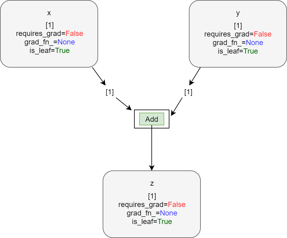
x = torch.ones(1, 1)
print(x.requires_grad, x.grad_fn, x.is_leaf)
y = torch.ones(1, 1)
print(y.requires_grad, y.grad_fn, y.is_leaf)
z = x + y
print(z)
print(z.requires_grad, z.grad_fn, z.is_leaf)
# z.backward() # will give runtime error

False None True
False None True
tensor([[2.]])
False None True

The last line will give RunTime error because the tensor does not have grad_fn and therefore we cannot calculate the gradients backward. As the tensors x and y have requires_grad=False, therefore, z has the same attribute.

The following diagram will make things even clearer.

Now, let’s carry out tensor operations with requires_grad=True and see how it affects the final output.

x = torch.ones(1, 1, requires_grad=True)
print(x.requires_grad, x.grad_fn, x.is_leaf)
y = torch.ones(1, 1, requires_grad=True)
print(y.requires_grad, y.grad_fn, y.is_leaf)
z = x + y
print(z)
print(z.requires_grad, z.grad_fn, z.is_leaf)
z.backward()
print(z)

True None True
True None True
tensor([[2.]], grad_fn=AddBackward0)
True AddBackward0 object at 0x00000139AECED108 False
tensor([[2.]], grad_fn=AddBackward0)

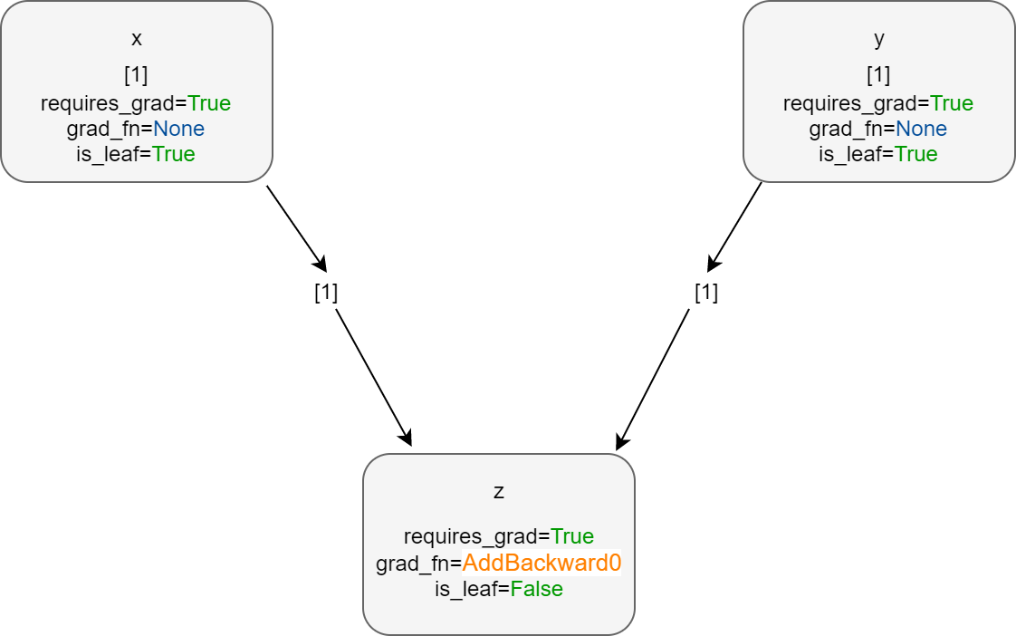
As both the tensors, x and y have requires_grad=True, so we can backpropagate through the resulting tensor z. You can also see that is_leaf is True for x and y. Also, z has requires_grad=True.

Summary and Conclusion

This ends the basics of autograd package in PyTorch. I hope that you liked this article. From the next article, we will focus on neural networks in PyTorch.