

PyTorch helps in carrying out deep learning projects and experiments with much ease. But we can improve the deep learning experience even more by tracking our training results, images, graphs and plots. For that, we can use TensorBoard. TensorBoard really eases out the task of keeping track of our deep learning projects. In this article, we will learn how to use TensorBoard with PyTorch for tracking deep learning projects and neural network training.
Introduction
When I first started to use TensorBoard along with PyTorch, then I started working on some online tutorials. The most common one that I found on the internet is in the original PyTorch tutorials. Everything was as seamless as expected.
The tutorial covers some basic but really important topics of using TensorBoard. These are the ones that you will need to track any deep learning project. Starting from visualizing images to tracking your training plots, everything is there.
But there is only one problem. Everything is covered using the very popular FashionMNIST dataset. Then I thought of giving it a try using the colored CIFAR10 images. My idea was that changing a few lines of code including the network architecture and the color channels will do the trick. But then I faced many other problems which we will cover shortly.
After that, I could not find many other better tutorials that used PyTorch along with TensorBoard along with colored images. And most of those did not explain some small yet very important tricks and codes.
So, in this article, we will cover the following things.
- How to use PyTorch with TensorBoard for tracking your deep learning project?
- We will use colored CIFAR10 images.
- How to correctly visualize colored images in TensorBoard?
- How to track training loss and accuracy of your deep learning project using TensorBoard?
Installing TensorBoard
If you already have TensorBoard installed, then you can skip this step. If you need to install TensorBoard, you can type the following command in your terminal to install it.
pip install tensorboard
Now, that the TensorBoard installation is ready, let’s start writing our code. Our main focus will be to know how to use TensorBoard with PyTorch. So, I may not go into many details of the other code parts. Still, I will provide an explanation wherever required. Now, many of you may be familiar with the initial steps, so, you can use the code directly.
Importing Modules
First, let’s import all the modules that we will require along the way.
# imports
import matplotlib.pyplot as plt
import numpy as np
import torch
import torchvision
import torchvision.transforms as transforms
import torch.nn as nn
import torch.nn.functional as F
import torch.optim as optim

from torch.utils.tensorboard import SummaryWriter
Some of the important modules include:
SummaryWriter: this is the TensorBoard module that PyTorch provides. We will be able to access all its functionalities after creating an object ofSummaryWriter.torchvision: we can download PyTorch datasets and access thetransformsusing this module.torch.nn: provides all the neural network layers that we will need.
Define the Data Transforms and Prepare the Dataset
Here, we will define the data preprocessing/transforms, and prepare the dataset as well.
The following code defines the transforms that we will apply to the CIFAR10 images.
# transforms
transform = transforms.Compose(
    [transforms.ToTensor(),
    transforms.Normalize((0.5, 0.5, 0.5), (0.5, 0.5, 0.5))])
The above code will convert all the image pixels into PyTorch tensors, and normalize the pixel values as well.
Next up, we can prepare our dataset.
# datasets
trainset = torchvision.datasets.CIFAR10('./data',
    download=True,
    train=True,
    transform=transform)
testset = torchvision.datasets.CIFAR10('./data',
    download=True,
    train=False,
    transform=transform)
trainloader = torch.utils.data.DataLoader(trainset, batch_size=4,
                                        shuffle=True, num_workers=2)
testloader = torch.utils.data.DataLoader(testset, batch_size=4,
                                        shuffle=False, num_workers=2)
Starting from line 2, first, we get our trainset and testset ready. If the data is already in the data directory, then it will directly load from there. Else the data will be downloaded. Then from line 10 till line 13, we prepare the trainloader and testloader of our dataset. The batch size is 4 in our example.
The CIFAR10 data contains images of 10 classes. The following code bock defines those classes in a tuple so that we can use them later.
# classes
classes = ('plane', 'car', 'bird', 'cat',
           'deer', 'dog', 'frog', 'horse', 'ship', 'truck')
Setting up TensorBoard
To write information into TensorBoard, we need to set it up by an object of SummaryWriter.
writer = SummaryWriter('runs/cifar10')
When you run the python code file, then a runs directory will be created in your present working directory. Inside runs, we define another directory called cifar10, which will store all the information that we write to TensorBoard. We can simply say that the above line of code creates runs/cifar10 directory. You will get to see how to use it in a short while.
Adding Images to TensorBoard
We can use TensorBoard to visualize images. SummaryWriter provides add_image() function which we can use to add an image to TensorBoard.
CIFAR10 images are colored images with 3 channels. We need to properly visualize and unnormalize the images before adding them to TensorBoard. The following is a helper function for the proper visualization of CIFAR10 images.
# to get and show proper images
def show_img(img):
    # unnormalize the images
    img = img / 2 + 0.5
    npimg = img.numpy()
    plt.imshow(np.transpose(npimg, (1, 2, 0)))
    return npimg # return the unnormalized images
In the above show_img() function (takes an image tensor as a parameter), first, we unnormalize the images (line 4). This is a very important step for TensorBoard visualization. If we do not unnormalize the images, then the images will be a lot noisy with random pixels. Then we convert the images to NumPy array and plot the images (lines 5 and 6). Finally, we return the unnormalized images. We return the image here, otherwise, we will again have to unnormalize them before passing them to add_img(). That would be a repetition of code and we want to avoid that.
Now, let’s call the show_img() function and add the images to TensorBoard.
# get images
dataiter = iter(trainloader)
images, labels = dataiter.next()

# create grid of images
img_grid = torchvision.utils.make_grid(images)

# get and show the unnormalized images
img_grid = show_img(img_grid)

# write to tensorboard
writer.add_image('cifar10 images', img_grid)
First, we get a random batch of 4 images from our trainloader (lines 2 and 3). Then we make a grid of the image using torchvision.utils.make_grid() which is a PyTorch tensor. At line 9 we call the show_img() function to plot the images and store the unnormalized images in img_grid. At line 12 we use the add_image() function to add the images to TensorBoard. It takes two arguments as inputs. One is a string defining the name of the images, and the other is the image itself.
Using TensorBoard
To visualize the images that we have added to TensorBoard you need to run a simple command in the terminal from your present working directory. Type the following command in the terminal.
tensorboard --logdir=runs
After a few seconds, it will tell you to go to http://localhost:6006/. So, open the localhost link in your browser and you will see something like the following.
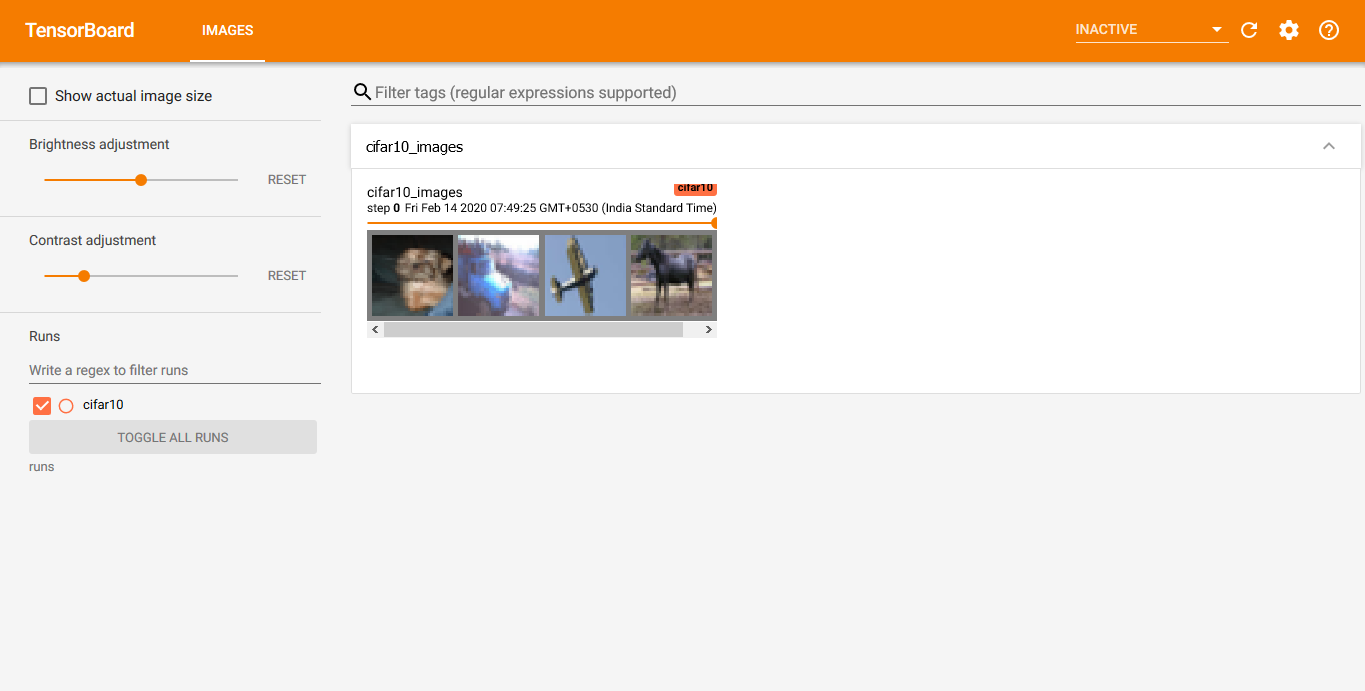
Click on the Images tab on the top and you should see a grid of four CIFAR10 images. You can run your code file as many times as you want and just refresh the TensorBoard tab to view the newly added images.
A bit ago we discussed how we need to unnormalize the images to properly view the images in TensorBoard. But what happens when you do not unnormalize the images. Suppose that skip the unnormalizing code. Then you will get a very output in your TensorBoard tab. Something very similar to the following.

There is also one other to avoid such noisy images in TensorBoard. You can clip the pixel values so that they will be within the range [0.0, 1.0]. For that, you add the following line of code.
img_grid = np.clip(img_grid, 0., 1.)
But in my opinion, unnormalizing the images and using them is a better idea as we can avoid the above code.
Adding a Deep Neural Network Graph to TensorBoard
We can also add a neural network graph to TensorBoard. This can help us to visualize all the connections and weight flows in our deep neural network.
Before adding the neural network graph to TensorBoard, we first need to define our neural network architecture.
The following is a very simple neural network architecture that we are using from the PyTorch tutorials.
class Net(nn.Module):
    def __init__(self):
        super(Net, self).__init__()
        self.conv1 = nn.Conv2d(3, 6, 5)
        self.pool = nn.MaxPool2d(2, 2)
        self.conv2 = nn.Conv2d(6, 16, 5)
        self.fc1 = nn.Linear(16 * 5 * 5, 120)
        self.fc2 = nn.Linear(120, 84)
        self.fc3 = nn.Linear(84, 10)

    def forward(self, x):
        x = self.pool(F.relu(self.conv1(x)))
        x = self.pool(F.relu(self.conv2(x)))
        x = x.view(-1, 16 * 5 * 5)
        x = F.relu(self.fc1(x))
        x = F.relu(self.fc2(x))
        x = self.fc3(x)
        return x

net = Net()

criterion = nn.CrossEntropyLoss()
optimizer = optim.SGD(net.parameters(), lr=0.001, momentum=0.9)
We will not go deep into the architectural details in this article. Simply speaking, we are initializing our Net() class with a net object. And we are using CrossEntropyLoss along with the SGD optimizer. Still, if you want, you can visit this article to know more about neural network architecture in PyTorch in detail.
To add a neural network graph to TensorBoard, we can use the add_graph() function.
writer.add_graph(net, images)
writer.close()
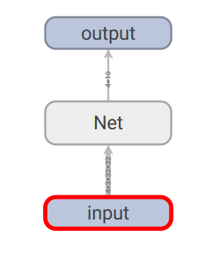
In the above code block, you can see that the add_graph() function takes two arguments. One is the net object and the other is the images tensor that we have defined before. If you refresh your TensorBoard tab now, you will an additional Graph tab on top. Click on it and you will see something similar to the following.
You can also expand each of the nodes by double-clicking on them.
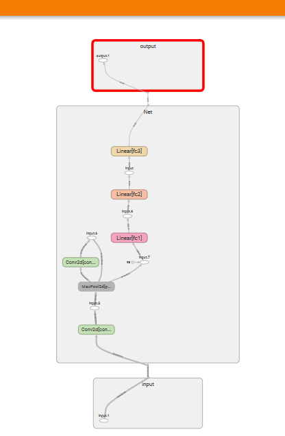
Expanding the neural network graph will show all the data flows in much more detail.
Tracking Neural Network Training with TensorBoard
This is probably one of the best uses of TensorBoard. You can track the accuracy and loss plots of your neural network as it is being trained.
Plotting the training accuracy and loss values to TensorBoard will give you a pretty good idea of how well the neural network is performing.
So, let’s get to writing down the code for tracking the training of our neural network with TensorBoard.
The following is the whole code of training our neural network along with TensorBoard logging.
for epoch in range(10):
    running_loss = 0.0
    running_correct = 0
    for data in (trainloader):

        # get the images and labels
        inputs, labels = data

        # set the parameter gradients to zero
        optimizer.zero_grad()

        outputs = net(inputs)
        loss = criterion(outputs, labels)
        _, preds = torch.max(outputs.data, 1)
        loss.backward()
        # update the parameters
        optimizer.step()
        running_loss += loss.item()
        running_correct += (preds == labels).sum().item()

    # log the epoch loss
    writer.add_scalar('training loss',
                    running_loss/len(trainset),
                    epoch)
    # log the epoch accuracy
    writer.add_scalar('training accuracy',
                    running_correct/len(trainset),
                    epoch)


    print(f"Epoch {epoch+1} train loss: {running_loss/len(trainset):.3f} train acc: {running_correct/len(trainset)}")
print('Finished Training')
We are training the neural network for 10 epochs. First, inside the for loop, we define running_loss and running_correct (lines 2 and 3). These two variables will help us keep track and calculate the epoch wise loss and accuracy.
Then we iterate through the trainloader for each epoch. inputs and labels store the images and the corresponding labels. At line 10, we set the parameter gradients to zero as we do not want the gradients to be adding up for each batch. Then we predict the outputs at line 12 and calculate the loss at line 13. preds stores the prediction of our neural network. At line 15 we backpropagate the gradients. After updating the gradients at line 17 we calculate the loss and accuracy.
After each epoch, we log the training loss and accuracy into TensorBoard. We can use the add_scalar() function for that. add_scalar() function takes three arguments. The first one is a string defining the name of the graph, the second one is the y-axis value, and the third is the x-axis value. In our case, the y-axis and x-axis are either the loss value or accuracy and the epoch number respectively.
Training and Accuracy Plots in TensorBoard
You can go to the Scalar tab in TensorBoard to visualize the plots.
The following two images show the training accuracy and loss plots that are saved from TensorBoard.
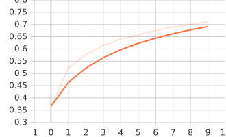
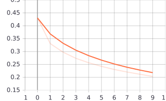
You can observe two very faint (ghost lines) along with the plots. Those two lines show the actual plot points. The deeper lines show the path which is due to the smoothing of the plots. You can use the Smoothing option on the right-hand side of the TensorBoard Scalar tab. That slider applies some smoothing to the lines so that the plots do not look much erratic.
Tracking Model Testing
For the final step, let’s now test our model on the testloader and track it with TensorBoard.
The following is the code for model testing.
class_correct = list(0. for i in range(10))
class_total = list(0. for i in range(10))
with torch.no_grad():
    for data in testloader:
        images, labels = data
        outputs = net(images)
        _, predicted = torch.max(outputs, 1)
        correct = (predicted == labels).squeeze()
        for i in range(4):
            label = labels[i]
            class_correct[label] += correct[i].item()
            class_total[label] += 1
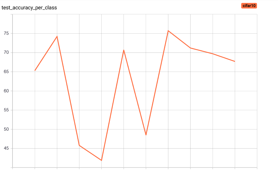
What we are actually doing is counting the correct prediction for each of the classes and saving it in class_correct. We will use that to plot a histogram showing the percentage of accuracy for each of the classes.
For getting the percentage distributions, we will the add_histogram() function.
for i in range(10):
    writer.add_histogram('test accuracy per class', 100 * class_correct[i] / class_total[i], i)
    print('Accuracy of %5s : %2d %%' % (
        classes[i], 100 * class_correct[i] / class_total[i]))
writer.close()
Accuracy of plane : 65 %
Accuracy of   car : 74 %
Accuracy of  bird : 45 %
Accuracy of   cat : 41 %
Accuracy of  deer : 70 %
Accuracy of   dog : 48 %
Accuracy of  frog : 75 %
Accuracy of horse : 71 %
Accuracy of  ship : 69 %
Accuracy of truck : 67 %
After executing the above code, you will find two more tabs in the TensorBoard window. One is Distributions and the other one is Histogram.
Taking a look at the Distributions plot of accuracy for each class.
And the Histogram is giving the following output.
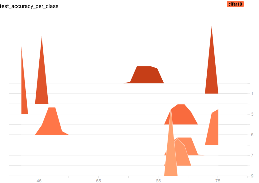
We are not getting much accuracy, but you can always train a bigger neural network to achieve better accuracy.
Summary and Conclusion
I hope that you are able to get the concepts and benefits of using TensorBoard to track your deep learning project. It can be a very useful tool to accurately track your neural network training and testing. Feel free to leave your thoughts in the comment section.
Resources
You can take a look at the following resources to gain more knowledge.
You can contact me using the Contact section. You can also find me on LinkedIn, and X.
