A Practical Guide to Build Robust Deep Neural Networks by Adding Noise

In this article, we will get hands-on experience on how to build robust deep neural networks by adding noise to the input data.

One of my previous articles was Adding Noise for Robust Deep Neural Network Models. It explained how neural networks suffer while generalizing when we add noise to the data. And how we can avoid such situations by training deep neural networks on noisy data. But it was a theoretical article summarizing the results of a few research papers.

Then there is another article Adding Noise to Image Data for Deep Learning Data Augmentation. This article explains how to add noise to the image data using Python and Scikit-Image. This article can give you a hands-on experience of adding different types of noise to image data and saving it on disk as well. In particular, you will learn to add three different types of noise:

• Gaussian noise.
• Salt and Pepper noise.
• Speckle Noise.

Now, this article is going to be much more practical. We will learn through code, how to achieve better generalization results of neural networks on noisy data.

If you are new to the topic, then you should surely read my previous article. It laid out many theoretical foundations about the problem and summarized a few research papers as well. Broadly, you will find the answers to the following questions in my previous article.

• Why Noise is Problem for Neural Networks?
• How Adding Noise to Inputs Help Neural Networks?
• Different Types of Noise.

So, in this article, we will try to write the code for replicating some of the results.

Our Approach for This Project

The Dataset

We will use the CIFAR10 image dataset for all of our experiments in this article. The main reason is that being colored images, this dataset will provide us with enough complexity to know whether we are successful or not. Moreover, it contains a variety of images.

The Neural Network Model

For the neural network model, we will use a ResNet18 model from PyTorch torch vision models. We will not use the ImageNet weights. Instead, we will initialize the model with random weights and fully train the model on our dataset.

By now, you must have guessed that we will be using the PyTorch deep learning library in this article. PyTorch makes it really easy to carry out deep learning experiments.

Type of Noise that We Will Add to the Data

Using PyTorch, we can easily add random noise to the CIFAR10 image data. In deep learning, one of the most important things is to able to work with tensors, NumPy arrays, and matrices easily. And PyTorch provides very easy functionalities for such things. Therefore, PyTorch is one of the best choices for carrying out deep learning research experiments.

So, all in all, we will be adding random noise to our data using PyTorch.

An Example of Random Noisy CIFAR10 Data

The following image shows an example of random noise added to CIFAR10 data.

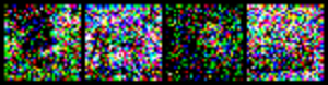
After adding noise, we can hardly recognize any of the images. This is going to be a good challenge for our deep neural network model.

Directory Structure of Our Project

To successfully manage everything, we will need a proper directory structure for this project. It is always a good practice to have a proper directory structure when carrying out deep learning experiments and projects. This ensures that nothing gets mixed and remains in place.

So, our directory structure is going to be like the following.

├───input
  │   └───data
  ├───outputs
  │   ├───models
  │   └───plots
  │
  └───src
      │   train_rnd_noise.py

input directory will contain the dataset that PyTorch datasets module will download. All the outputs will go into the outputs directory. It has two subdirectories. models will contain all the trained models that we will save and plots will contain our training/validation accuracy and loss plots. src will contain the python file that we will execute through the command line.

Steps to Confirm our Experiments

So, how are we going to carry out the implementation? If we think in a very basic way, then we will be adding noise to both, the training data and the validation data. We will try four different methods to confirm the experiment.

• First, we will train and validate without adding any noise. This should give us the highest accuracies in both, training and validation.
• Then we will add noise to the training data only. This should give us less accuracy than when training without any noise.
• After that, we will train on clean images, and validate on noisy images. We should get less validation accuracy than the previous methods.
• Finally, we will train and validate on noisy images. This should give us more accuracy than training on clean images and validating on noisy images.

Also, we will be using argument parser for providing the number of epochs, and whether or not to add noise to training and validation data. Let’s start writing the code.

Importing Libraries and Modules

Let’s import all the required libraries and modules that we will need for this project.

import torch
import torchvision
import torchvision.transforms as transforms
import torch.nn as nn
import torch.nn.functional as F
import torch.optim as optim
import torchvision.models as models
import numpy as np
import matplotlib.pyplot as plt
import time
import argparse
import matplotlib
plt.style.use('ggplot')

from torchvision import datasets

Going over all the important imports:

• torch: as we will be implementing everything using the PyTorch deep learning library, so we import torch first.
• torchvision: this module will help us download the CIFAR10 dataset, pre-trained PyTorch models, and also define the transforms that we will apply to the images.
• torch.nn: we will get access to all the neural network layers through torch.nn.
• torch.optim: this will help us define the optimizer of our choice.
• argparse: for defining our argument parsers.
• matplotlib: for saving the plots after training and validation.

Define the Argument Parsers

Here, we will define the argument parsers. We will use argument parsers while executing the python code file through the terminal.

ap = argparse.ArgumentParser()
ap.add_argument('-e', '--epochs', type=int, default=10,
	help='number of epochs to train the model')
ap.add_argument('-n_tr', '--train_noise', default='no', type=str,
    help='whether to add noise to training data or not')  
ap.add_argument('-n_te', '--test_noise', default='no', type=str,
    help='whether to add noise to training data or not')  
args = vars(ap.parse_args())

We are using three arguments for the command line execution. --epochs for the number of epochs that we want to train our model for. It has a default value of 10. --train_noise and --test_noise specify whether we want to add random noise to our training and validation data or not. Both of these are strings and we will be passing them as yes or no. Both of these are set to no by default.

Defining argument parsers for deep learning projects can be really useful. They will allow us to train our neural network with different parameters without hardcoding them.

Defining Transforms and Helper Function to Get the Computation Device

Image Transforms

Applying image transforms is one of the most important steps in deep learning when working with image data. Correctly applying transforms to the image data can help us improve the results a lot.

Remember that we will be using the ResNet18 model from PyTorch models. Well, if you visit the PyTorch hub ResNet documentation, you will find the normalization for the pixel values should be mean = [0.485, 0.456, 0.406] and std = [0.229, 0.224, 0.225]. Therefore, we will be using these values as well. Also, we will be converting all the pixel values to tensors. The following code defines the transforms.

transform = transforms.Compose([
    transforms.ToTensor(),
    transforms.Normalize(mean=[0.485, 0.456, 0.406],
                          std=[0.229, 0.224, 0.225]),
])

In the above code block, at line 2 we are converting all the pixel values to PyTorch tensors. And at line 3, we are normalizing the pixel values as PyTorch ResNet models expect it.

Helper Function to Get the Computation Device

Now, let’s write a helper function to get the computation device for our neural network operations. The following code will return either the CPU or the CUDA GPU device depending upon availability.

# get computation device
def get_device():
    if torch.cuda.is_available():
        device = 'cuda:0'
    else:
        device = 'cpu'
    return device
device = get_device()

The following are some parameters that we will be using along the way as we write our code.

Some Important Parameters

# parameters
batch_size = 32
num_classes = 10
pretrained = False
requires_grad = True

Line 2 initializes the batch size. Here, the batch size is set as 32. You can either increase or decrease the batch size depending upon your computation power. However, a batch size of 32 should not be a problem for the CIFAR10 dataset. Then we have num_classes which is set to 10. It is the number of classes in the dataset.

The next two (lines 4 and 5) parameters are a bit important. We will be using the ResNet18 model. While initializing the neural network model, we can specify whether we want to use pre-trained weights or not. If we set it to True, then the pre-trained ImageNet weights will be downloaded. Setting pretrained = False will initialize the neural network model with random weights.

Again, we can also specify whether or not we want to train those weights. requires_grad = True will make the neural network model to learn the weights while training. And requires_grad = False will keep those hidden layer weights as frozen, only updating the classification layer weights.

For our purpose, we will be initializing the model with random weights and learning those weights during training as well.

Preparing the Data

To download the data, we will use the torchvision.datasets module. It provides many datasets and CIFAR10 is one of them.

# get the data
trainset = datasets.CIFAR10(
    root='input/data',
    train=True,
    download=True, 
    transform=transform
)
trainloader = torch.utils.data.DataLoader(
    trainset, 
    batch_size=batch_size,
    shuffle=True
)
testset = datasets.CIFAR10(
    root='input/data',
    train=False,
    download=True,
    transform=transform
)
testloader = torch.utils.data.DataLoader(
    testset, 
    batch_size=batch_size,
    shuffle=False
)

For the trainset and testset, we have set the path to input/data. Either the CIFAR10 dataset is already there, else it will be downloaded. Also, we are applying the transform to the trainset and the testset.

To prepare the iterable data loaders, we are using the DataLoader module from PyTorch. The batch_size is as defined above.

Prepare the Deep Neural Network Model

This part is going to be very important. We will prepare our deep neural network model here. Obviously, we will be using the ResNet18 model, but still, we need to make some important design choices.

Let’s write the python code first, then we will go to the explanation part.

def model():
    model = models.resnet18(progress=True, pretrained=pretrained)
    # freeze hidden layers
    if requires_grad == False:
        for param in model.parameters():
            param.requires_grad = False
    # train the hidden layers
    elif requires_grad == True:
        for param in model.parameters():
            param.requires_grad = True
    # make the classification layers learnable
    model.fc = nn.Linear(512, num_classes)
    
    model = model.to(device)
    
    return model
model = model()

We are naming the function to prepare the neural network model as model(). In the above code block, line 2 initializes the ResNet18 neural network model. One of the parameters is pretrained that we have set to pretrained which corresponds to False that we have defined earlier. Therefore, the model will be initialized with random weights instead of the ImageNet weights. This will allow us to train our model from scratch.

Next, starting from line 3 till line 10 we are defining whether we want to update the hidden layer weights or not. In our case, we have set required_grad = True, so, it will execute the lines 8 to 10.

model.parameters() contains all the hidden layer parameters. To access those parameters we can simply use a for loop. And to make those weights learnable, we can set requires_grad = True (line 10).

Whether we update the hidden layer weights or not, but we have to change the classification layer to our use case. By default, most of the pre-trained models have an output dimensionality of 1000 classes. We have to change that to the number of classes that is present in our dataset. Line 12 does that for us. It is also called as making the classification layer learnable. For our use case, we are setting the out_features as num_classes which is set to 10.

At line 14 we loading the model to the computation device and return it at line 16. Finally, at line 17, we call the model() function.

Define the Loss Function and the Optimizer

For the loss function, we will use the CrossEntropyLoss(). And the optimizer is going to be SGD().

# loss function
criterion = nn.CrossEntropyLoss()
# optimizer
optimizer = optim.SGD(model.parameters(), lr=0.001, momentum=0.9)

The learning rate for optimizer is 0.001 with a momentum of 0.9.

The Training Function

During training our neural network, we will print some useful information on the screen. This information will give us an easier understanding of whether all the parameters are as per our choice or not.

# the training function
print(f"Training with noise: {args['train_noise']}")
print(f"Validating with noise: {args['test_noise']}")
print(f"pretrained = {pretrained}, requires_grad = {requires_grad}")
if pretrained and requires_grad:
    print('Training with ImageNet weights and updating hidden layer weights')
elif pretrained and not requires_grad:
    print('Training with ImageNet weights and freezing hidden layers weights')
elif not pretrained and requires_grad:
    print('Training with random weights and updating hidden layers weights')
elif not pretrained and not requires_grad:
    print('Training with random weights and freezing hidden layers weights')
def train(NUM_EPOCHS, epoch, model, dataloader):
    model.train()
    loss = 0
    acc = 0
    running_loss = 0.0
    running_correct = 0
    for i, data in enumerate(trainloader):
        img, labels = data[0].to(device), data[1].to(device)
        # add noise to the image data
        if args['train_noise'] == 'yes':
            noise = torch.randn(img.shape).to(device)
            new_img = img + noise
        elif args['train_noise'] == 'no':
            new_img = img
        new_img = new_img.to(device)
        optimizer.zero_grad()
        outputs = model(new_img)
        loss = criterion(outputs, labels)
        _, preds = torch.max(outputs.data, 1)
        running_loss += loss.item()
        running_correct += (preds == labels).sum().item()
        # backpropagation
        loss.backward()
        # update the parameters
        optimizer.step()
               
    loss = running_loss / len(trainset)
    acc = 100. * running_correct / len(trainset)
    print(f"Epoch {epoch+1} of {NUM_EPOCHS}, train loss: {loss:.3f}, train acc: {acc:.3f}")
    return loss, acc

Lines 2 and 3 will print whether we are adding any noise to the train and validation set or not. Then from lines 4 to 12, it will print whether are using ImageNet weights or not. It will also print whether we are updating the hidden layer parameters or not. In the future, if you ever consider changing those parameters, then you will have an easier way to verify the correctness while training.

The train() function starting from line 13 takes 4 parameters, the total number of epochs, the current epoch, the model, and the data loader. First, we define four variables, loss, acc, running_loss, and running_correct. These will help us keep track of our losses and accuracies both per epoch and per iteration of the data loader.

From line 19, we start to iterate through the data loader. We get the img and labels from the data loader. Then, starting from line 21 till 26, we decide whether we want to add random noise to our image data or not. The decision is based on the arguments provided while executing the program. We call the changed image as new_img.

At line 28 we set the parameter gradients to zero. Then we calculate the outputs and loss in the next two lines. At line 32 we find out the predictions for the batch and then add the loss and number of correct predictions for the current batch. At line 35 and 37, we carry out the backpropagation and update the parameter gradients.

After each epoch, we are calculating the loss and accuracy and printing them as well. Finally, we return the loss and accuracy for that epoch.

The Validation Function

During validation, we will not be updating any parameter or backpropagating the gradients.

# the validation function
def validate(NUM_EPOCHS, epoch, model, testloader):
    model.eval()
    loss = 0.0
    acc = 0
    running_loss = 0.0
    running_correct = 0
    with torch.no_grad():
        for i, data in enumerate(testloader):
            img, labels = data[0].to(device), data[1].to(device)
            # add noise to the image data
            if args['test_noise'] == 'yes':
                noise = torch.randn(img.shape).to(device)
                new_img = img + noise
            elif args['test_noise'] == 'no':
                new_img = img
            new_img = new_img.to(device)
            outputs = model(new_img)
            loss = criterion(outputs, labels)
            _, preds = torch.max(outputs.data, 1)
            running_loss += loss.item()
            running_correct += (preds == labels).sum().item()

    loss = running_loss / len(testset)
    acc = 100. * running_correct / len(testset)
    print(f"Epoch {epoch+1} of {NUM_EPOCHS}, val loss: {loss:.3f}, val acc: {acc:.3f}")
    return loss, acc 

Everything remains inside a with torch.no_grad() block so that the gradients do not get calculated. We carry on the same as the training function. But we do not update the parameters or backpropagate the gradients.

Executing the Functions, Saving the Model and Plots

This is the final section involving code. We will execute all of the above functions first.

train_loss, train_acc = [], []
val_loss, val_acc = [], []
start = time.time()
for epoch in range(args['epochs']):
    e_start = time.time()
    train_epoch_loss, train_epoch_acc = train(args['epochs'], epoch, model, trainloader)
    train_loss.append(train_epoch_loss)
    train_acc.append(train_epoch_acc)
    val_epoch_loss, val_epoch_acc = validate(args['epochs'], epoch, model, testloader)
    val_loss.append(val_epoch_loss)
    val_acc.append(val_epoch_acc)
    e_end = time.time()
    print(f"Took {(e_end-e_start)/60:.3f} minutes for epoch {epoch+1}")
end = time.time()
print(f"Took {(end-start)/60:.3f} minutes to train")

First, we are defining four lists, train_loss, train_acc, val_loss, and val_acc. They will save the loss values and the accuracies of train() and validate() respectively. Then at line 3, we are defining a start time that ends at line 14. This will track the total training time for our neural network model.

From line 4 we start to train our neural network model inside a for loop for the specified number of epochs that we get from the argument parser. Inside we have e_start and e_end(lines 5 and 12) to track the epoch wise time taken. After that, from lines 6 to 11 we are just executing the functions and appending the losses and accuracies per epoch into the lists.

Saving the Models and Plots

Here, we will write the code to save the neural network model that we have trained and the plots that we generate after training.

torch.save(model, f"outputs/models/{args['train_noise']}_{args['test_noise']}.pth")
plt.figure()
plt.plot(train_acc, label='training accuracy')
plt.plot(val_acc, label='validation accuracy')
plt.title('Accuracy Plots')
plt.xlabel('Accuracy')
plt.ylabel('Epochs')
plt.legend()
plt.savefig(f"outputs/plots/{args['train_noise']}_{args['test_noise']}_acc.png")
plt.figure()
plt.plot(train_loss, label='training loss')
plt.plot(val_loss, label='validation loss')
plt.title('Loss Plots')
plt.xlabel('Loss')
plt.ylabel('Epochs')
plt.legend()
plt.savefig(f"outputs/plots/{args['train_noise']}_{args['test_noise']}_loss.png")

The model goes inside the outputs/model directory and all the plots go inside the outputs/plots directory. The naming convention that we are using is a bit odd but convenient for our use case.

We are naming models and plots using the amount of noise that we trained the neural network model on. For the models it is args['train_noise']}_{args['test_noise']}.pth. So, if we train the model using no noise for both training and validation, then it will be saved as no_no.pth.

For the plots, it is followed by an extra _acc.png or _loss.png depending on which plot it is. For example, for no noise, the accuracy plot will save as no_no_acc.png.

Executing the train_rnd_noise.py File

It is time to execute the python file. We will train our model four times using four different sets of noise.

• No train noise, no validation noise.
• With train noise, no validation noise.
• No train noise, with validation noise.
• With train noise, with validation noise.

To train the neural network model, execute the following commands in the command line. Obviously you will have to wait for one training to complete before you can move onto the next.

python src/train_rnd_noise.py --epochs=20 --train_noise=no --test_noise=no

Training with noise: no
Validating with noise: no
pretrained = False, requires_grad = True
Training with random weights and updating hidden layers weights
Epoch 1 of 20, train loss: 0.049, train acc: 43.878
Epoch 1 of 20, val loss: 0.041, val acc: 53.370
Took 1.211 minutes for epoch 1
...
Epoch 20 of 20, train loss: 0.002, train acc: 97.334
Epoch 20 of 20, val loss: 0.045, val acc: 70.770
Took 1.271 minutes for epoch 20
Took 25.555 minutes to train

python src/train_rnd_noise.py --epochs=20 --train_noise=yes --test_noise=no

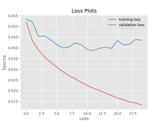
Training with noise: yes
Validating with noise: no
pretrained = False, requires_grad = True
Training with random weights and updating hidden layers weights
Epoch 1 of 20, train loss: 0.052, train acc: 39.678
Epoch 1 of 20, val loss: 0.053, val acc: 39.490
Took 1.293 minutes for epoch 1
...
Epoch 20 of 20, train loss: 0.013, train acc: 84.766
Epoch 20 of 20, val loss: 0.043, val acc: 60.550
Took 1.261 minutes for epoch 20
Took 25.494 minutes to train

python src/train_rnd_noise.py --epochs=20 --train_noise=no --test_noise=yes

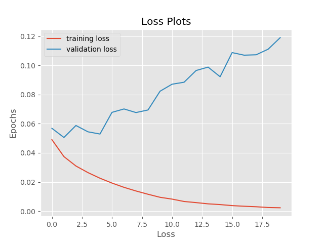
Training with noise: no
Validating with noise: yes
pretrained = False, requires_grad = True
Training with random weights and updating hidden layers weights
Epoch 1 of 20, train loss: 0.049, train acc: 43.384
Epoch 1 of 20, val loss: 0.057, val acc: 39.320
Took 1.211 minutes for epoch 1
...
Epoch 20 of 20, train loss: 0.002, train acc: 97.312
Epoch 20 of 20, val loss: 0.119, val acc: 45.570
Took 1.277 minutes for epoch 20
Took 24.740 minutes to train

python src/train_rnd_noise.py --epochs=20 --train_noise=yes --test_noise=yes

Training with noise: yes
Validating with noise: yes
pretrained = False, requires_grad = True
Training with random weights and updating hidden layers weights
Epoch 1 of 20, train loss: 0.052, train acc: 40.178
Epoch 1 of 20, val loss: 0.044, val acc: 48.410
Took 1.296 minutes for epoch 1
... 
Epoch 20 of 20, train loss: 0.013, train acc: 84.790
Epoch 20 of 20, val loss: 0.040, val acc: 63.730
Took 1.320 minutes for epoch 20
Took 26.119 minutes to train

Analyzing Our Results and Plots

In this section, we will analyze all the results and plots that have been generated while training four of the neural network model.

No Train Noise, No Validation Noise

The following images show the first set of plots that we get after training.

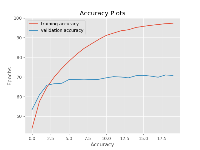
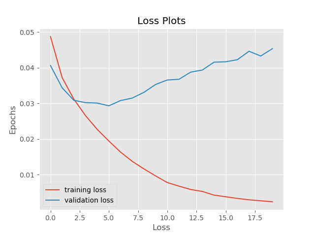
The accuracy plot shows that after 20 epochs of training, we are getting more than 97% of training accuracy and 71% of validation accuracy. The validation accuracy may have increased if we trained for longer.

But the story of loss plot is somewhat different. The training loss is decreasing as expected, but we see that the validation loss is increasing after 10 epochs. This is a classic sign of our neural network overfitting the data. Maybe adding noise to the data will make it overfit less.

Let’s see what the other results say.

With Training Noise, No Validation Noise

Here are the results of our second run, with training noise but no validation noise.

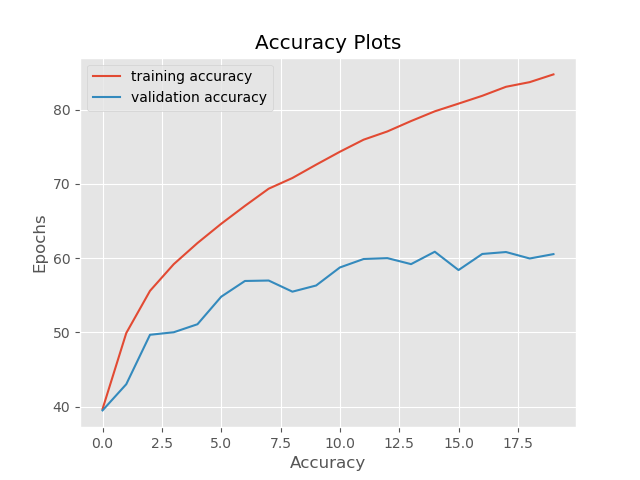
In this case, the training accuracy is much worse due to the presence of noise, around 84%. The validation accuracy is even worse with 60% accuracy. Most probably, this is the case, as the training examples are noisy and are a lot different from the validation examples. Therefore, the neural network is taking a lot longer to learn the patterns.

Moving on to the loss plot, both, the training loss and validation loss are more than before. Moreover, validation loss is much more erratic. This is the case as the neural network only trained on noisy images and did not validate on them.

No Training Noise, with Validation Noise

Let’s take a look at the plots where we do not train on noisy images but validate on noisy images.

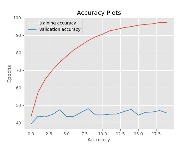
As expected, here the results are the worst. We are not training on the noisy data but our neural network tries to validate on them. The train and validation images are a lot different. Even though we have a 97% training accuracy, the validation accuracy is only 45%.

Similarly, the validation loss reaches as high as 0.12 because of the noisy images.

With Training Noise, with Validation Noise

This is the last case where we both train and validate on noisy images.

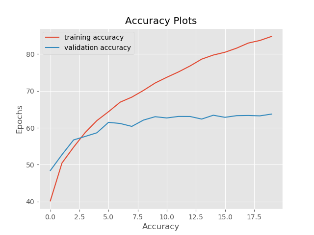
These are the results that we want to focus on the most. The training accuracy with noise reaches around 85% which is less than without any noise. But the important thing is that the validation accuracy reaches 63% which we would not have got if we would not have trained on noisy images. This shows that the neural network model learns to identify images even though noise is present. We can say that the model is at least somewhat robust to noisy images now.

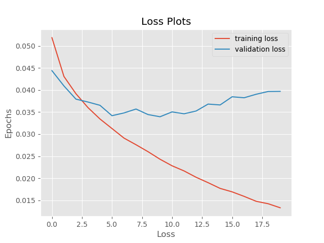
The training loss also reaches 0.013 and the validation noise is 0.040. So, the loss results are also better after we train and validate the model on noisy images.

But we can see that even in the final case (and most of the other) the model is overfitting. The loss plots clearly show that. So, what can we do to avoid that?

Some Ways to Avoid Overfitting

The following are some of the methods to avoid overfitting while building robust deep neural network models.

• Get more training and validation data.
• Apply noise to only a certain percentage of images chosen randomly at training and validation time.
• Create a totally new data set by applying noise. In that case, we will have two datasets, one clean and another noisy. So, the dataset size will be doubled and we will have much more data to train and validate on.

Summary and Conclusion

In this article, you learned how to build robust neural network models by adding noise to the image data. Hopefully, we were able to somewhat replicate the results of the three research papers that we discussed in the previous articles. I hope that this article acts as a practical complementary guide for those articles. You can leave any thoughts or doubts in the comment section and will try my best to address them.

You can contact me using the Contact section. You can also find me on LinkedIn, and Twitter.