Visualizing Filters and Feature Maps in Convolutional Neural Networks using PyTorch

When dealing with image data in deep learning, then convolutional neural networks (CNN) are the go-to architectures. Convolutional neural networks have proved to provide many state-of-the-art solutions and benchmarks in deep learning and computer vision. Image recognition, object detection, and semantic segmentation are only some of the applications of convolutional neural networks among many more.

But when it comes down to how a convolutional neural network decides what an image actually is, things become trickier. The question can be in many forms:

• How did the neural network decide that the image is a cat?
• Why did the image classify a cat as a bird?
• What did the convolutional neural network see in the intermediate layers?

After many years of research, we can answer some of the questions, and some other questions partially. This is in contrast to machine learning model explainability. When dealing with machine learning models like random forests, or decision trees, we can explain many of its decision making procedure. Data scientists and business managers also need to know why a model took a particular decision as it can radically affect a big organization.

In regard to deep neural networks, explainability is still a widely researched field. Many businesses avoid the use of neural network models due to a lack of such explainability.

But we can answer some of the questions that we asked above. When dealing with deep convolutional networks, we have two very efficient ways to know what a model sees. They are filters and feature maps. Further on, in this article, we will learn the following things corresponding to convolutional neural networks:

• What are filters in CNN?
• What are feature map in CNN?
• How to visualize filters and feature maps in convolutional neural networks?

What are Filters in Convolutional Neural Networks?

When we talk about filters in convolutional neural networks, then we are specifically talking about the weights. If you do a lot of practical deep learning coding, then you may know them by the name of kernels. I hope that you get the analogy now. And you must have used kernel size of 3×3 or maybe 5×5 or maybe even 7×7.

These filters will determine which pixels or parts of the image the model will focus on. Now, how do we determine which part of the image will the model focus on? We will obviously answer that question but when we will visualize the filters in one of the later sections.

For now, let’s take a look at how a 7×7 filter will look like in a convolutional neural network.

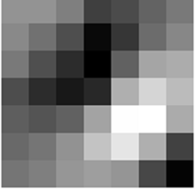
Figure 1 shows a 7×7 filter from the ResNet-50 convolutional neural network model. To be specific, it is a filter from the very first 2D convolutional layer of the ResNet-50 model.

Such filters will determine what pixel values of an input image will that specific convolutional layer focus on.

I hope that now, you have some idea about filters in convolutional neural networks.

What are Feature Maps in Convolutional Neural Networks?

Feature maps are what we get after a filter has passed through the pixel values of an input image. Specifically, it is what the convolutional layer sees after passing the filters on the image. It is what we call a convolution operation in terms of deep learning

For example, let’s consider that we have an image of a cat and we pass a 7×7 filter on that image. Then, maybe we will get something similar to the following image after the convolution operation.

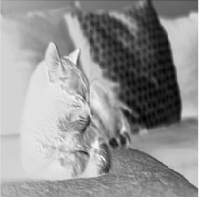
If you observe closely, then in figure 2, you will find that some parts of the image are dark while others are bright. I think that you have somehow managed to guess the reason. This because of the values the 7×7 filters and which parts of the filter are dark, and which are light.

Can We Visualize All the Filters and Feature Maps in a Model?

The real question is, can we visualize all the convolved feature maps in a neural network model. The simple answer is yes.

We will go through all the steps of visualizing the filters and features maps in detail.

Visualizing Filters and Feature Maps in Convolutional Neural Networks

In this section, we will look into the practical aspects and code everything for visualizing filters and feature maps.

The Convolutional Neural Network Model

We will use the PyTorch deep learning library in this tutorial.

Note: If you need to know the basics of a convolutional neural network in PyTorch, then you may take look at my previous articles.

To carry on further, first, we need to a convolutional neural network model. We will use the ResNet-50 neural network model for visualizing filters and feature maps. Along with that, we will load the pre-trained ImageNet weights.

Actually, using a ResNet-50 model for visualizing filters and feature maps is not very ideal. The reason is that the ResNet models, in general, are complex. Traversing through the inner convolutional layers can become quite difficult. Then again, this is the very reason for choosing the ResNet-50 model. You will learn how to access the inner convolutional layers of a difficult architecture. In the future, you will feel much more comfortable when working with similar or simpler architectures.

The Image that We will Use

We will use the following cat image in this tutorial. Go ahead, and download this image.

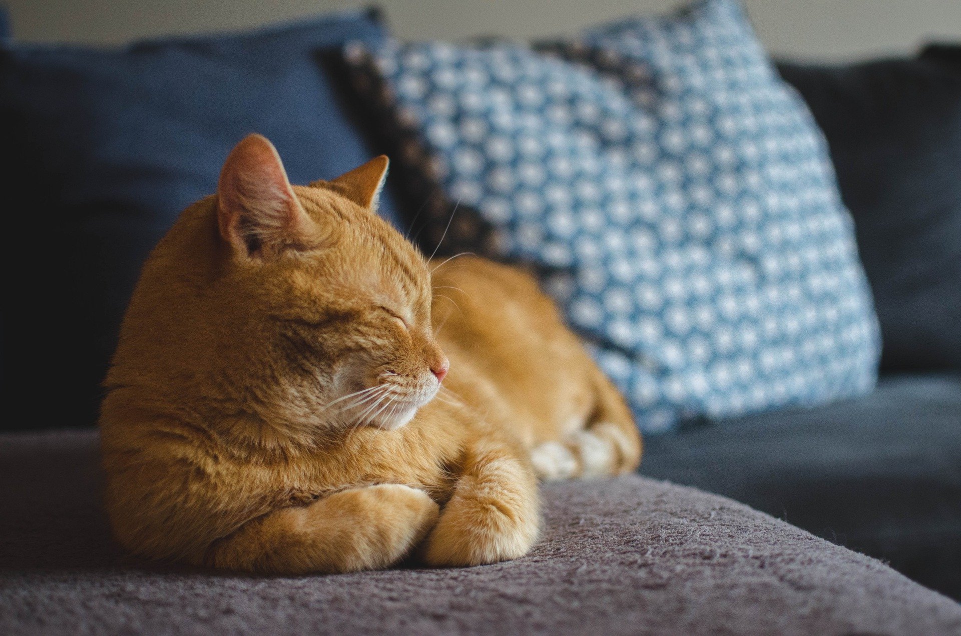
After downloading the image, name it as cat.jpg.

We will use the following folder structure in this tutorial.

├───input
│       cat.jpg
│
├───outputs
└───src
    │   filters_and_maps.py

• input directory has the original cat.jpg image.
• In outputs, we will save all the filters and features maps that we are going to visualize.
• src contains the filters_and_maps.py file in which we will write all our code.

Now, we are all set to start coding to visualize filters and feature maps in ResNet-50.

From here on, all the code that we will write will go into the filters_and_maps.py file.

Importing the Required Modules and Libraries

Let’s import all the libraries and modules first. We will not need many, just a few important ones.

import torch
import matplotlib.pyplot as plt
import numpy as np
import torch.nn as nn
import cv2 as cv
import argparse

from torchvision import models, transforms

• matplotlib to display and save the filters and feature map images.
• torch.nn will give access to the hidden convolutional layers of the ResNet-50 model.
• Using cv2 we will read the image.
• argparse for parsing the arguments that we will provide through the command line. We will provide the name of the image through the command line.
• torchvision to access the ResNet-50 model and transforms to transform the input image.

Next, we will build an argument parser and parse the command line argument. For the command-line argument, we will only provide the name of the image. The following block of code builds the argument parser and parses through the arguments.

ap = argparse.ArgumentParser()
ap.add_argument('-i', '--image', required=True,
    help='path to image')
args = vars(ap.parse_args())

Load the ResNet-50 Model

In this section, we will load the ResNet-50 model from torchvision.models module.

# load the model
model = models.resnet50(pretrained=True)
print(model)

model_weights = [] # we will save the conv layer weights in this list
conv_layers = [] # we will save the 49 conv layers in this list

# get all the model children as list
model_children = list(model.children())

Going through the above code block.

• Line 2 loads the ResNet-50 model. Note that we are also loading the pre-trained ImageNet weights. This will allow us to get better visualizations without training the convolutional neural network.
• We are creating two lists at lines 5 and 6. model_weights will save the weights of all the convolutional layers and conv_layers will save all the convolutional layers. It is important to remember that the ResNet-50 model has 50 layers in total. 49 of those layers are convolutional layers and a final fully connected layer. In this tutorial, we will only work with the 49 convolutional layers.
• At line 9, we are getting all the model children as list and storing them in the model_children list. This will allow us to easily access the hidden layers.

Accessing all the Convolutional Layers and Their Weights

We will have to save all the convolutional layers and the respective weights. As discussed earlier, we will save them in conv_layer and model_weights respectively.

This section might feel a bit complex as we will have to go through a lot of hidden layers and sequences. Other models like VGG nets are not that much complex. But then again, you will learn a lot by using the ResNet-50 model. Let’s take a look at the ResNet-50 model first. If you print the model that you have loaded above, then you will get the following output.

ResNet(
  (conv1): Conv2d(3, 64, kernel_size=(7, 7), stride=(2, 2), padding=(3, 3), bias=False)
  (bn1): BatchNorm2d(64, eps=1e-05, momentum=0.1, affine=True, track_running_stats=True)
  (relu): ReLU(inplace=True)
  (maxpool): MaxPool2d(kernel_size=3, stride=2, padding=1, dilation=1, ceil_mode=False)
  (layer1): Sequential(
    (0): Bottleneck(
      (conv1): Conv2d(64, 64, kernel_size=(1, 1), stride=(1, 1), bias=False)
      (bn1): BatchNorm2d(64, eps=1e-05, momentum=0.1, affine=True, track_running_stats=True)
      (conv2): Conv2d(64, 64, kernel_size=(3, 3), stride=(1, 1), padding=(1, 1), bias=False)
      (bn2): BatchNorm2d(64, eps=1e-05, momentum=0.1, affine=True, track_running_stats=True)
      (conv3): Conv2d(64, 256, kernel_size=(1, 1), stride=(1, 1), bias=False)
      (bn3): BatchNorm2d(256, eps=1e-05, momentum=0.1, affine=True, track_running_stats=True)
      (relu): ReLU(inplace=True)
      (downsample): Sequential(
        (0): Conv2d(64, 256, kernel_size=(1, 1), stride=(1, 1), bias=False)
        (1): BatchNorm2d(256, eps=1e-05, momentum=0.1, affine=True, track_running_stats=True)
      )
    )
    (1): Bottleneck(
      (conv1): Conv2d(256, 64, kernel_size=(1, 1), stride=(1, 1), bias=False)
      (bn1): BatchNorm2d(64, eps=1e-05, momentum=0.1, affine=True, track_running_stats=True)
      (conv2): Conv2d(64, 64, kernel_size=(3, 3), stride=(1, 1), padding=(1, 1), bias=False)
      (bn2): BatchNorm2d(64, eps=1e-05, momentum=0.1, affine=True, track_running_stats=True)
      (conv3): Conv2d(64, 256, kernel_size=(1, 1), stride=(1, 1), bias=False)
      (bn3): BatchNorm2d(256, eps=1e-05, momentum=0.1, affine=True, track_running_stats=True)
      (relu): ReLU(inplace=True)
...
(2): Bottleneck(
      (conv1): Conv2d(2048, 512, kernel_size=(1, 1), stride=(1, 1), bias=False)
      (bn1): BatchNorm2d(512, eps=1e-05, momentum=0.1, affine=True, track_running_stats=True)
      (conv2): Conv2d(512, 512, kernel_size=(3, 3), stride=(1, 1), padding=(1, 1), bias=False)
      (bn2): BatchNorm2d(512, eps=1e-05, momentum=0.1, affine=True, track_running_stats=True)
      (conv3): Conv2d(512, 2048, kernel_size=(1, 1), stride=(1, 1), bias=False)
      (bn3): BatchNorm2d(2048, eps=1e-05, momentum=0.1, affine=True, track_running_stats=True)
      (relu): ReLU(inplace=True)
    )
  )
  (avgpool): AdaptiveAvgPool2d(output_size=(1, 1))
  (fc): Linear(in_features=2048, out_features=1000, bias=True)

I have clipped the output in between so that it does not take a lot of space. Still, you can see that there nestings of Bottleneck layers within different layers, starting from layer1 to layer4.

We will have to traverse through all these nestings to retrieve the convolutional layers and their weights.

The following code shows how to retrieve all the convolutional layers and their weights.

# counter to keep count of the conv layers
counter = 0 

# append all the conv layers and their respective weights to the list
for i in range(len(model_children)):
    if type(model_children[i]) == nn.Conv2d:
        counter += 1
        model_weights.append(model_children[i].weight)
        conv_layers.append(model_children[i])
    elif type(model_children[i]) == nn.Sequential:
        for j in range(len(model_children[i])):
            for child in model_children[i][j].children():
                if type(child) == nn.Conv2d:
                    counter += 1
                    model_weights.append(child.weight)
                    conv_layers.append(child)
print(f"Total convolutional layers: {counter}")

• First, at line 2, we initialize a counter variable to keep track of the number of convolutional layers.
• Starting from line 5, we are going through all the layers of the ResNet-50 model.
• Specifically, we are checking for convolutional layers at three levels of nesting:
  • Line 6, checks if any of the direct children of the model is a convolutional layer.
  • Then from line 10, we check whether any of the Bottleneck layer inside the Sequential blocks contain any convolutional layers.
• If any of the above two conditions satisfy, then we append that child node and the weights to the conv_layers and model_weights respectively,

If you want, then you can also print the saved convolutional layers and the weights using the following code.

# take a look at the conv layers and the respective weights
for weight, conv in zip(model_weights, conv_layers):
    # print(f"WEIGHT: {weight} \nSHAPE: {weight.shape}")
    print(f"CONV: {conv} ====> SHAPE: {weight.shape}")

Visualizing Convolutional Layer Filters

In this section, we will visualize the convolutional layer filters. For the sake of simplicity, we will only visualize the filters of the first convolutional layer.

# visualize the first conv layer filters
plt.figure(figsize=(20, 17))
for i, filter in enumerate(model_weights[0]):
    plt.subplot(8, 8, i+1) # (8, 8) because in conv0 we have 7x7 filters and total of 64 (see printed shapes)
    plt.imshow(filter[0, :, :].detach(), cmap='gray')
    plt.axis('off')
    plt.savefig('../outputs/filter.png')
plt.show()

• We are iterating through the weights of the first convolutional layer (starting from line 3).
• The output is going to be 64 filters of 7×7 dimensions. The 64 refers to the number of hidden units in that layer.
• At line 7, we are saving the filter plot as filter.png.

Now, running the python file from the src folder as

python filters_and_maps.py --image cat.jpg

you will get the following output.

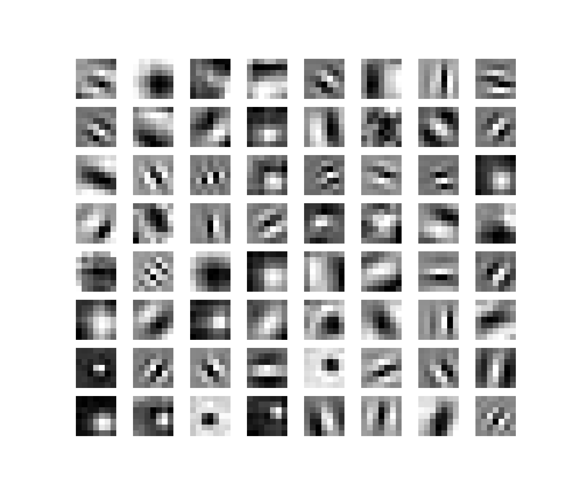
We can see in figure 4 that there are 64 filters in total. And each filter is 7×7 shape. This 7×7 is the kernel size for the first convolutional layer.

You may notice that some patches are dark and others are bright. We know that pixel values range from 0 to 255. 0 corresponds fully black color, and 255 corresponds to the white color. This means that the dark patches have a lower weight than the brighter patches.

When the affine transformations take place with the input image, then the white patches will be more responsible for the activation of that part of the image. In simple words, the model will focus more on the area of the image where the weight values are more when doing the element-wise product of the weights with the pixel values.

Next, let’s prepare our image for visualizing the feature maps.

Reading the Image and Defining the Transforms

We have already parsed the image argument through the argument parser. Now, we just need to read the image using OpenCV. Also, for the transforms, we will simply use PyTorch transforms module. We just need to convert the image into PIL format, resize it and then convert it to tensor.

# read and visualize an image
img = cv.imread(f"../input/{args['image']}")
img = cv.cvtColor(img, cv.COLOR_BGR2RGB)
plt.imshow(img)
plt.show()

# define the transforms
transform = transforms.Compose([
    transforms.ToPILImage(),
    transforms.Resize((512, 512)),
    transforms.ToTensor(),
])

img = np.array(img)
# apply the transforms
img = transform(img)
print(img.size())
# unsqueeze to add a batch dimension
img = img.unsqueeze(0)
print(img.size())

• After defining the transforms, we are converting the image into a NumPy array at line 14.
• Then we apply the transforms at line 16.
• Line 19 unsqueezes the image to add an extra batch dimension.

Adding the batch dimension is an important step. Now the size of the image, instead of being [3, 512, 512], is [1, 3, 512, 512], indicating that there is only one image in the batch.

Visualizing the Feature Maps of the Convolutional Layers

Visualizing the feature maps of the image after passing through the convolutional layers of the ResNet-50 model consists of two steps.

• Passing the image through each convolutional layer and saving each layer’s output.
• Visualizing the feature map blocks of each layer.

Before moving further, I would like to point out that visualizing the feature maps is not really necessary when doing any neural network projects. But if you are carrying out any large scale projects or writing a novel research paper, especially in the computer vision field, then it is very common to analyze the feature maps.

When reading deep learning computer vision research papers, then you may have noticed that many authors provide activation maps for the input image. This is specifically to show which part of the image activates that particular layer’s neurons in a deep neural network model. This gives the authors as well as the reader a good idea of what the neural network sees.

Passing the Input Image Through Each Convolutional Layer

We will first give the image as an input to the first convolutional layer. After that, we will use a for loop to pass the last layer’s outputs to the next layer, until we reach the last convolutional layer.

# pass the image through all the layers
results = [conv_layers[0](img)]
for i in range(1, len(conv_layers)):
    # pass the result from the last layer to the next layer
    results.append(conv_layers[i](results[-1]))

# make a copy of the `results`
outputs = results

• At line 2, we give the image as input to the first convolutional layer.
• Then we iterate from through the second till the last convolutional layer using a for loop.
• We give the last layer’s output as the input to the next convolutional layer (results[-1]) (line 15).
• Also, we append each layer’s output to the results list.
• Finally, we make a copy of the results as save it as outputs (line 8) as we do not want to manipulate the original results.

Visualizing the Feature Maps

This is the final step. We will write the code to visualize the feature maps that we just saved.

Notice that the upper layers (near the fully connected layers) have many feature maps, in the range of 512 to 2048. But we will only visualize 64 feature maps from each layer as any more than that will make the outputs really cluttered.

The following code shows how to iterate through each layer’s output and save the feature maps.

# visualize 64 features from each layer 
# (although there are more feature maps in the upper layers)
for num_layer in range(len(outputs)):
    plt.figure(figsize=(30, 30))
    layer_viz = outputs[num_layer][0, :, :, :]
    layer_viz = layer_viz.data
    print(layer_viz.size())
    for i, filter in enumerate(layer_viz):
        if i == 64: # we will visualize only 8x8 blocks from each layer
            break
        plt.subplot(8, 8, i + 1)
        plt.imshow(filter, cmap='gray')
        plt.axis("off")
    print(f"Saving layer {num_layer} feature maps...")
    plt.savefig(f"../outputs/layer_{num_layer}.png")
    # plt.show()
    plt.close()

• Starting from line 3, we iterate through the outputs.
• Then we get layer_viz as outputs[num_layer][0, :, :, :] which are all the values of that corresponding layer (lines 6 and 7).
• We are printing the layer_viz size just for a sanity check.
• Starting from line 8, we iterate through the filters in each layer_viz. We break out of the loop if it is the 64\(^{th}\) feature map.
• From line 11 to 15, we plot the feature map, and save them to disk as well. I have commented out plt.show() (line 16) as we are saving the images and can analyze them later. You can uncomment that line if you want to visualize the images as the program executes.

Now, we need to run the python program from the src folder. You can again run it using the same command as before.

python filters_and_maps.py --image cat.jpg

Now, the images are saved to the disk and we are all set to analyze the results.

Analyzing the Outputs and Feature Maps

When running the python program, you will get lots of other outputs in the terminal apart from the images. We will be analyzing the saved feature maps in this section.

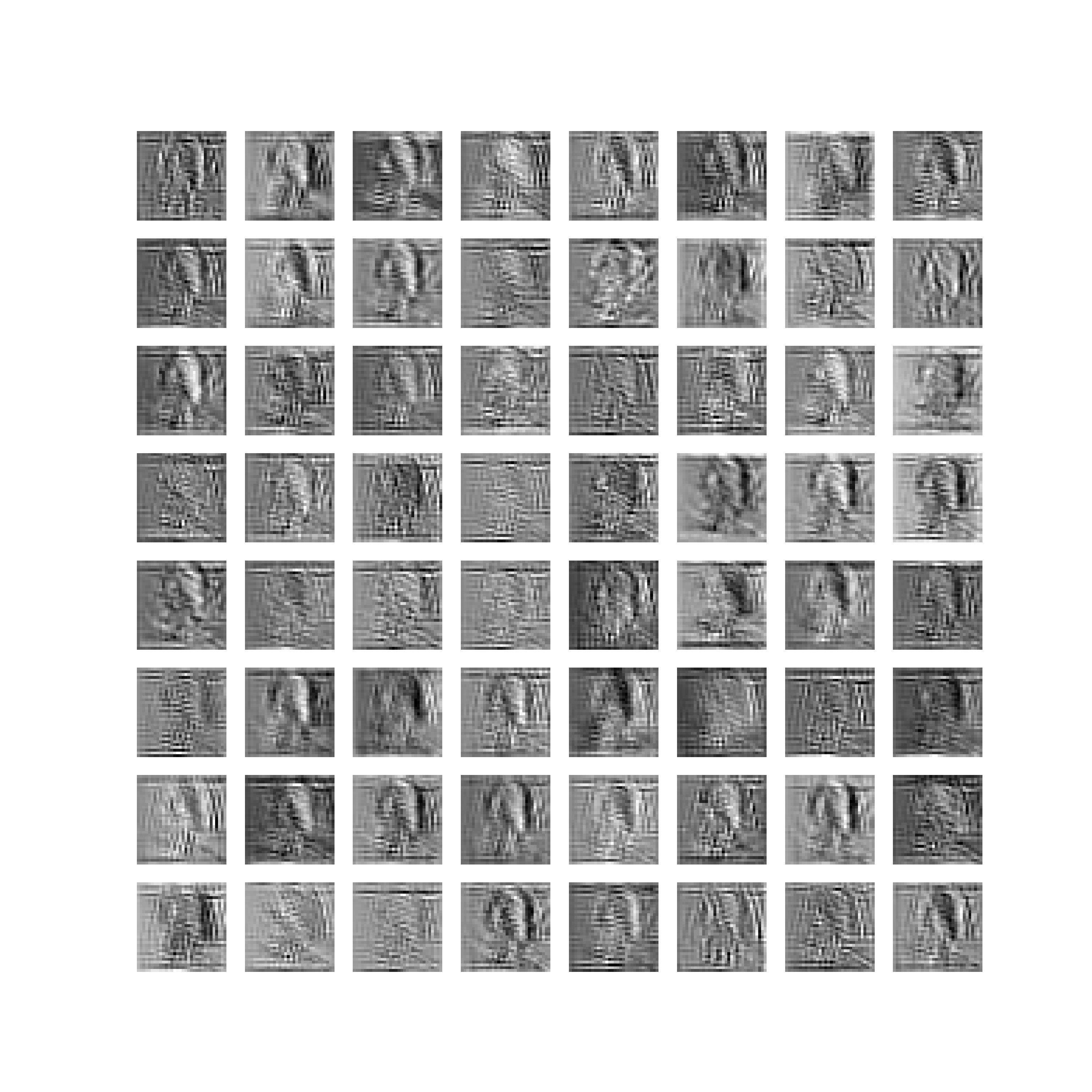
The following image shows the feature map from the first convolutional layer (layer 0).

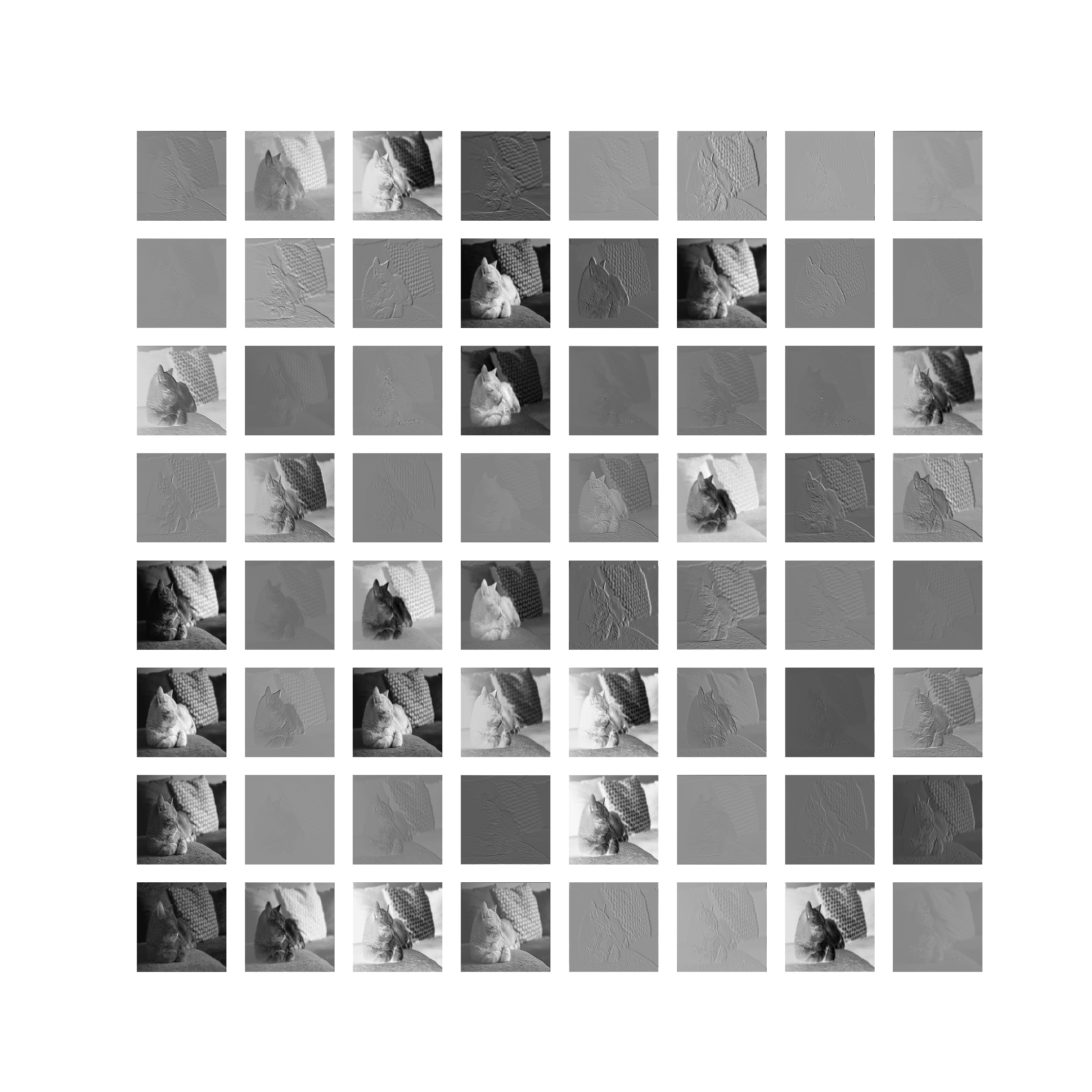
In figure 5, you can see that different filters focus on different aspects while creating the feature map of an image.

Some feature maps focus on the background of the image. Some others create an outline of the image. A few filters create feature maps where the background is dark but the image of the cat is bright. This is due to the corresponding weights of the filters. It is very clear from the above image that in the deep layers, the neural network gets to see very detailed feature maps of the input image.

Let’s take a look at a few other feature maps.

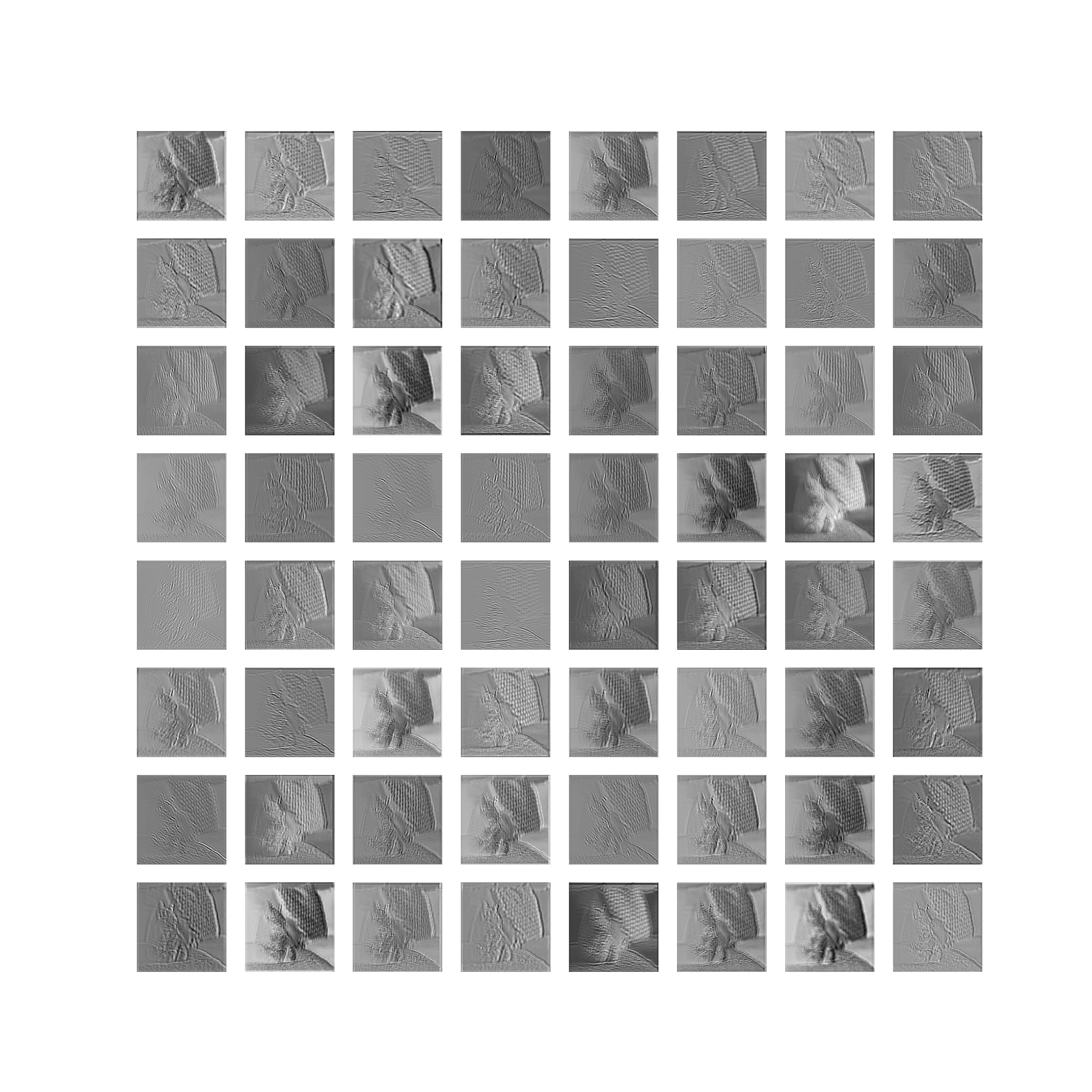
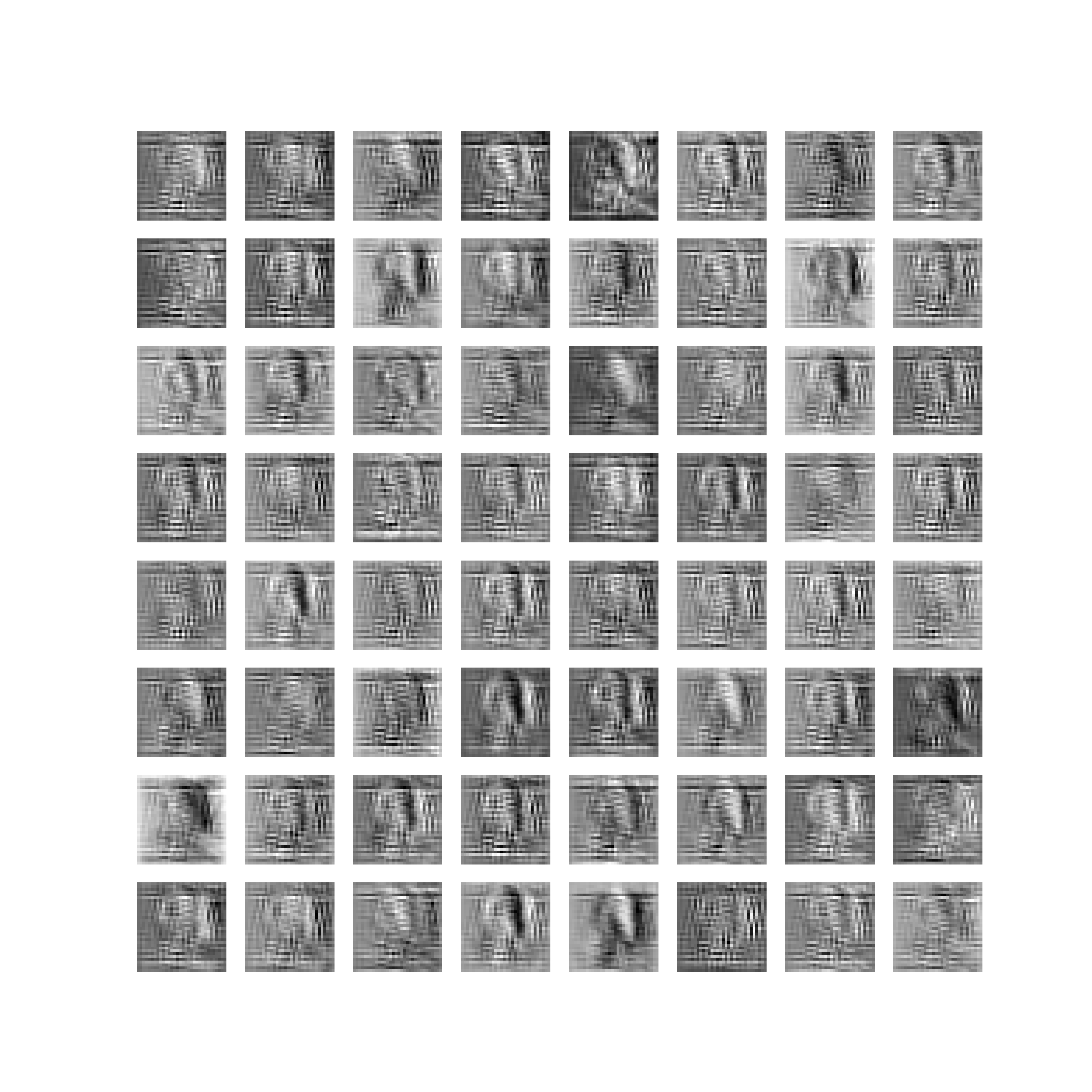
You can observe that as the image progresses through the layers then the details from the images slowly disappear. They look like noise, but surely there is a pattern in those feature maps which human eyes cannot detect, but a neural network can.

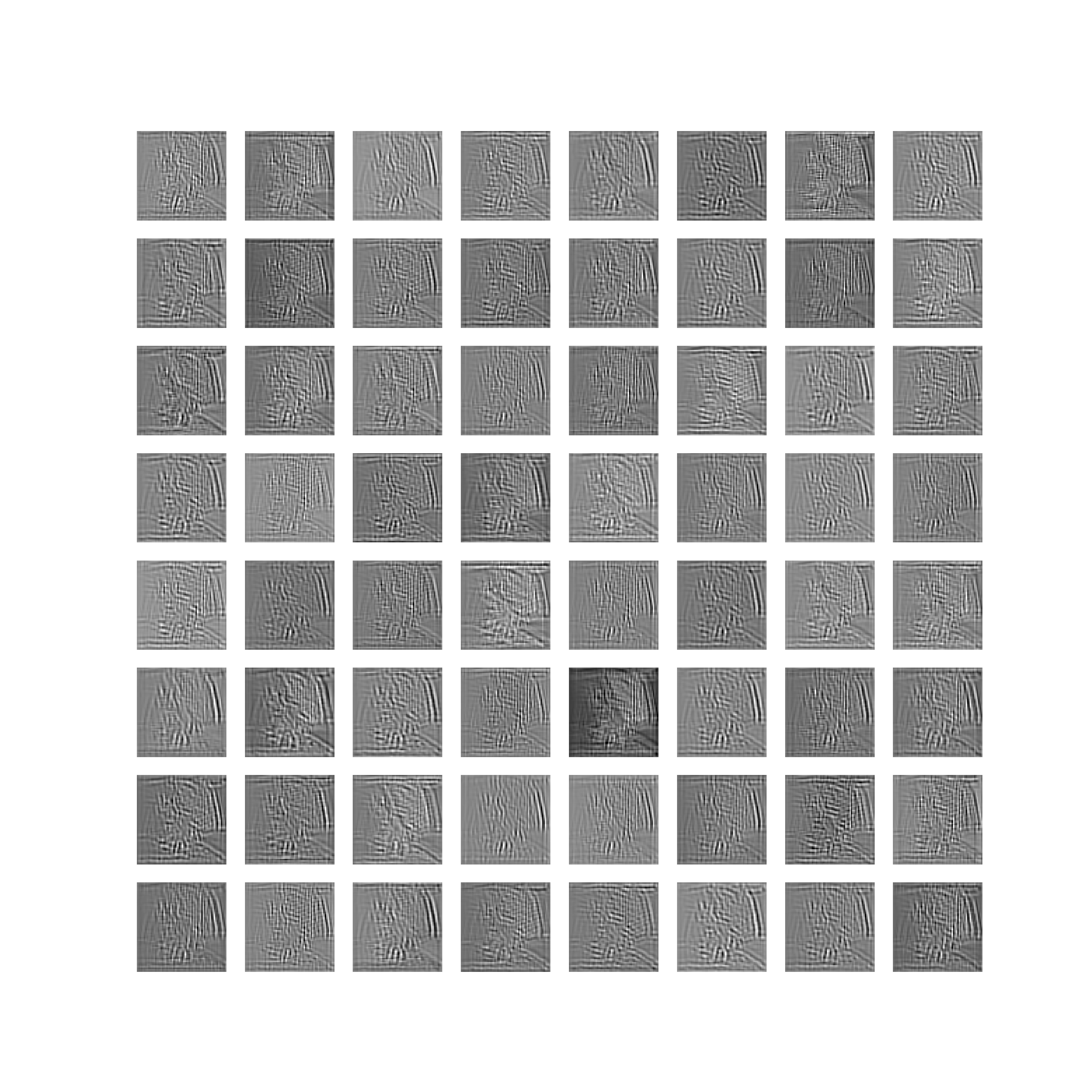
By the time the image reaches the last convolutional layer (layer 48) (figure 9), then it is impossible for a human being to tell that there is a cat in there. These last layer outputs are really important for the fully connected neurons which basically form the classification layers in a convolutional neural network.

More About Convolutional Neural Networks

If you want to learn more about convolutional neural networks, then the Convolutional Networks: Deep Learning is a great read. This chapter from the Deep Learning book by Ian Goodfellow, Yoshua Bengio and Aaron Courville is a must-read for anyone in the deep learning field.

Summary and Conclusion

In this article, you learned the following:

• What are filters and feature maps in convolutional neural networks?
• How to visualize the filters and features maps of a ResNet-50 model using PyTorch?
• How different feature maps from different layers look like in a convolutional neural network?

If you have any thoughts or suggestions, then feel free to use the comment section. I will try my best to address them

You can contact me using the Contact section. You can also find me on LinkedIn, and Twitter.