Sparse Autoencoders using KL Divergence with PyTorch

In this tutorial, we will learn about sparse autoencoder neural networks using KL divergence. We will also implement sparse autoencoder neural networks using KL divergence with the PyTorch deep learning library.

In the last tutorial, Sparse Autoencoders using L1 Regularization with PyTorch, we discussed sparse autoencoders using L1 regularization. We also learned how to code our way through everything using PyTorch.

This tutorial will teach you about another technique to add sparsity to autoencoder neural networks. Kullback-Leibler divergence, or more commonly known as KL-divergence can also be used to add sparsity constraint to autoencoders.

What Will We Cover in this Article?

• Sparsity in autoencoder.
• A brief on KL-divergence.
• How to use KL-divergence to implement sparsity in autoencoder neural networks?
• Coding a sparse autoencoder neural network using KL divergence sparsity with PyTorch.

We will go through all the above points in detail covering both, the theory and practical coding.

Before moving further, there is a really good lecture note by Andrew Ng on sparse autoencoders that you should surely check out. I will be using some ideas from that to explain the concepts in this article.

Sparsity in Autoencoders

In the previous articles, we have already established that autoencoder neural networks map the input \(x\) to \(\hat{x}\).

But bigger networks tend to just copy the input to the output after a few iterations. We want to avoid this so as to learn the interesting features of the data. We can do that by adding sparsity to the activations of the hidden neurons.

In neural networks, a neuron fires when its activation is close to 1 and does not fire when its activation is close to 0. So, adding sparsity will make the activations of many of the neurons close to 0.

What is KL Divergence?

KL divergence is a measure of the difference between two probability distributions. When two probability distributions are exactly similar, then the KL divergence between them is 0.

For example, let’s say that we have a true distribution \(P\) and an approximate distribution \(Q\). Then KL divergence will calculate the similarity (or dissimilarity) between the two probability distributions. The following is the formula:

$$
D_{KL}(P \| Q) = \sum_{x\epsilon\chi}P(x)\left[\log \frac{P(X)}{Q(X)}\right]
$$

where \(\chi\) is the probability space.

We need to keep in mind that although KL divergence tells us how one probability distribution is different from another, it is not a distance metric. That is, it does not calculate the distance between the probability distributions \(P\) and \(Q\).

All of this is all right, but how do we actually use KL divergence to add sparsity constraint to an autoencoder neural network? That’s what we will learn in the next section.

We will not go into the details of the mathematics of KL divergence. Instead, let’s learn how to use it in autoencoder neural networks for adding sparsity constraints.

Sparsity and KL Divergence

We already know that an activation close to 1 will result in the firing of a neuron and close to 0 will result in not firing.

Now, suppose that \(a_{j}\) is the activation of the hidden unit \(j\) in a neural network. When we give it an input \(x\), then the activation will become \(a_{j}(x)\). This is the case for only one input.

Let the number of inputs be \(m\). So, \(x\) = \(x^{(1)}, …, x^{(m)}\). Then we have the average of the activations of the \(j^{th}\) neuron as

$$
\hat\rho_{j} = \frac{1}{m}\sum_{i=1}^{m}[a_{j}(x^{(i)})]
$$

There is another parameter called the sparsity parameter, \(\rho\). This value is mostly kept close to 0. And we would like \(\hat\rho_{j}\) and \(\rho\) to be as close as possible. In other words, we would like the activations to be close to 0. That will prevent the neurons from firing.

Sparsity Penalty Along with Regular Cost Function

In neural networks, we always have a cost function or criterion. For autoencoders, it is generally MSELoss to calculate the mean square error between the actual and predicted pixel values.

We will add another sparsity penalty in terms of \(\hat\rho_{j}\) and \(\rho\) to this MSELoss. The penalty will be applied on \(\hat\rho_{j}\) when it will deviate too much from \(\rho\). The following is the formula for the sparsity penalty.

$$
\sum_{j=1}^{s} = \rho\ log\frac{\rho}{\hat\rho_{j}}+(1-\rho)\ log\frac{1-\rho}{1-\hat\rho_{j}}
$$

where \(s\) is the number of neurons in the hidden layer.

In terms of KL divergence, we can write the above formula as \(\sum_{j=1}^{s}KL(\rho||\hat\rho_{j})\). Here, \( KL(\rho||\hat\rho_{j})\) = \(\rho\ log\frac{\rho}{\hat\rho_{j}}+(1-\rho)\ log\frac{1-\rho}{1-\hat\rho_{j}}\).

After finding the KL divergence, we need to add it to the original cost function that we are using (i.e. the MSELoss). Let’s call that cost function \(J(W, b)\). So, the final cost will become

$$
J_{sparse}(W, b) = J(W, b) + \beta\ \sum_{j=1}^{s}KL(\rho||\hat\rho_{j})
$$

where \(\beta\) controls the weight of the sparsity penalty.

You will find all of these in more detail in these notes. Do give it a look if you are interested in the mathematics behind it.

Looks like this much of theory should be enough and we can start with the coding part.

Implementing a Sparse Autoencoder using KL Divergence with PyTorch

Beginning from this section, we will focus on the coding part of this tutorial and implement our through sparse autoencoder using PyTorch.

The Dataset and the Directory Structure

Like the last article, we will be using the FashionMNIST dataset in this article. Starting with a too complicated dataset can make things difficult to understand.

For the directory structure, we will be using the following one.

├───input
├───outputs
│   └───images
└───src
        sparse_ae_kl.py

• input will contain the Fashion MNIST dataset that we will download using the PyTorch datasets module.
• outputs will contain the model that we will train and save along with the loss plots. The images subdirectory will contain the images that the autoencoder neural network will reconstruct.
• src folder contains a python file named sparse_ar_kl.py. All of our code will go into this python file.

Importing the Required Modules

In this section, we will import all the modules that we will require for this project.

'''
USAGE:
python sparse_ae_kl.py --epochs 10 --reg_param 0.001 --add_sparse yes
'''

import torch
import torchvision
import torch.nn as nn
import matplotlib
import matplotlib.pyplot as plt
import torchvision.transforms as transforms
import torch.nn.functional as F
import torch.optim as optim
import os
import time
import numpy as np
import argparse

from tqdm import tqdm
from torchvision import datasets
from torch.utils.data import DataLoader
from torchvision.utils import save_image

matplotlib.style.use('ggplot')

Some of the important modules in the above code block are:

• torch.nn will allow us to access the PyTorch neural network layers like nn.Linear and many others.
• torchvision makes it really easier for us to download the predefined datasets and apply transforms to that data.
• torch.optim will allow us to access the optimizers like Adam.
• DataLoader will help us to create our own train and test loaders.
• save_image from torchvision.utils makes it easier to save the tensor images.
• argparse for defining and parsing the command line arguments.

Constructing the Argument Parsers and Setting the Parameters

Here, we will construct our argument parsers and define some parameters as well. Let’s start with constructing the argument parser first.

# constructing argument parsers 
ap = argparse.ArgumentParser()
ap.add_argument('-e', '--epochs', type=int, default=10,
	help='number of epochs to train our network for')
ap.add_argument('-l', '--reg_param', type=float, default=0.001, 
    help='regularization parameter `lambda`')
ap.add_argument('-sc', '--add_sparse', type=str, default='yes', 
    help='whether to add sparsity contraint or not')
args = vars(ap.parse_args())

We are parsing three arguments using the command line arguments. They are:

• --epochs define the number of epochs we want to train our autoencoder neural network for. The default value is 10.
• --reg_param is the weight parameter \(\beta\). We have set the default weight to 0.001.
• --add_sparse indicates whether we want to add the KL divergence sparsity penalty or not. This takes a string, either ‘yes’ or ‘no’. For this tutorial, this will be ‘yes’ of course.

Reading and initializing those command-line arguments for easier use. We will also initialize some other parameters like learning rate, and batch size.

EPOCHS = args['epochs']
BETA = args['reg_param']
ADD_SPARSITY = args['add_sparse']
RHO = 0.05
LEARNING_RATE = 1e-4
BATCH_SIZE = 32

print(f"Add sparsity regularization: {ADD_SPARSITY}")

Lines 1, 2, and 3 initialize the command line arguments as EPOCHS, BETA, and ADD_SPARSITY. We initialize the sparsity parameter RHO at line 4. The learning rate is set to 0.0001 and the batch size is 32.

If you want you can also add these to the command line argument and parse them using the argument parsers. Because these parameters do not need much tuning, so I have hard-coded them.

Define the Transforms and Prepare the Dataset

To define the transforms, we will use the transforms module of PyTorch. For the transforms, we will only convert data to tensors. The following code block defines the transforms that we will apply to our image data.

# image transformations
transform = transforms.Compose([
    transforms.ToTensor(),
])

The next block of code prepares the Fashion MNIST dataset.

trainset = datasets.FashionMNIST(
    root='../input/data',
    train=True, 
    download=True,
    transform=transform
)
testset = datasets.FashionMNIST(
    root='../input/data',
    train=False,
    download=True,
    transform=transform
)
 
# trainloader
trainloader = DataLoader(
    trainset, 
    batch_size=BATCH_SIZE,
    shuffle=True
)
#testloader
testloader = DataLoader(
    testset, 
    batch_size=BATCH_SIZE, 
    shuffle=False
)

• Starting from line 1 to line 12 we first prepare the trainset and testset. The FashionMNIST data will be downloaded into input/data folder. We are also applying the transform to the datasets.
• From line 14 to line 25, we prepare the iterable trainloader and testloader. We have set the BATCH_SIZE as 32. Shuffling is only applied to the trainloader and not to the testloader.

Most probably, if you have a GPU, then you can set the batch size to a much higher number like 128 or 256. That will make the training much faster than a batch size of 32.

Helper Functions

In this section, we will define some helper functions to make our work easier.

First, let’s define the functions, then we will get to the explanation part.

# get the computation device
def get_device():
    if torch.cuda.is_available():
        device = 'cuda:0'
    else:
        device = 'cpu'
    return device
device = get_device()

# make the `images` directory
def make_dir():
    image_dir = '../outputs/images'
    if not os.path.exists(image_dir):
        os.makedirs(image_dir)
make_dir()

# for saving the reconstructed images
def save_decoded_image(img, name):
    img = img.view(img.size(0), 1, 28, 28)
    save_image(img, name)

• First, at line 2, we define the function get_device() that either gets a hold on the CUDA GPU device or the CPU depending on the availability. For neural network training, it is always preferable to have a GPU.
• At line 11 we define the function make_dir(). This creates a folder images inside the ouputs folder where all the autoencoder reconstructed images will be saved.
• The final function, starting from line 18 is save_decoded_image(). This function takes an image tensor and a name string as input parameters. It will save the tensor values as images after resizing them to appropriate width and height.

This marks the end of some of the preliminary things we needed before getting into the neural network coding. We will begin that from the next section.

Define the Autoencoder Model

We will call our autoencoder neural network module as SparseAutoencoder(). The neural network will consist of Linear layers only. The following code block defines the SparseAutoencoder().

# define the autoencoder model
class SparseAutoencoder(nn.Module):
    def __init__(self):
        super(SparseAutoencoder, self).__init__()
 
        # encoder
        self.enc1 = nn.Linear(in_features=784, out_features=256)
        self.enc2 = nn.Linear(in_features=256, out_features=128)
        self.enc3 = nn.Linear(in_features=128, out_features=64)
        self.enc4 = nn.Linear(in_features=64, out_features=32)
        self.enc5 = nn.Linear(in_features=32, out_features=16)
 
        # decoder 
        self.dec1 = nn.Linear(in_features=16, out_features=32)
        self.dec2 = nn.Linear(in_features=32, out_features=64)
        self.dec3 = nn.Linear(in_features=64, out_features=128)
        self.dec4 = nn.Linear(in_features=128, out_features=256)
        self.dec5 = nn.Linear(in_features=256, out_features=784)
 
    def forward(self, x):
        # encoding
        x = F.relu(self.enc1(x))
        x = F.relu(self.enc2(x))
        x = F.relu(self.enc3(x))
        x = F.relu(self.enc4(x))
        x = F.relu(self.enc5(x))
 
        # decoding
        x = F.relu(self.dec1(x))
        x = F.relu(self.dec2(x))
        x = F.relu(self.dec3(x))
        x = F.relu(self.dec4(x))
        x = F.relu(self.dec5(x))
        return x
model = SparseAutoencoder().to(device)

• In the autoencoder neural network, we have an encoder and a decoder part. The encoder part (from line 7) starts with 784 in_fetures. This corresponds to the 28×28 number of pixels in the FashionMNIST images.
• Similarly, the decoder part (from line 13) starts with in_features of 16 and ends with out_features of 784.
• The encoding and decoding happens in the forward() function. All the layers are passed through the ReLU activation function.
• Line 35 loads the model onto the computation device.

We also need to define the optimizer and the loss function for our autoencoder neural network. For the loss function, we will use the MSELoss which is a very common choice in case of autoencoders. And for the optimizer, we will use the Adam optimizer.

# the loss function
criterion = nn.MSELoss()
# the optimizer
optimizer = optim.Adam(model.parameters(), lr=LEARNING_RATE)

The learning rate for the Adam optimizer is 0.0001 as defined previously.

Defining Sparsity Penalty and KL Divergence

This section perhaps is the most important of all in this tutorial. Here, we will implement the KL divergence and sparsity penalty. We will go through the details step by step so as to understand each line of code.

First, of all, we need to get all the layers present in our neural network model. That is just one line of code and the following block does that.

# get the layers as a list
model_children = list(model.children())

We get all the children layers of our autoencoder neural network as a list. Printing the layers will give all the linear layers that we have defined in the network.

Linear(in_features=784, out_features=256, bias=True)
Linear(in_features=256, out_features=128, bias=True)
Linear(in_features=128, out_features=64, bias=True)
Linear(in_features=64, out_features=32, bias=True)
Linear(in_features=32, out_features=16, bias=True)
Linear(in_features=16, out_features=32, bias=True)
Linear(in_features=32, out_features=64, bias=True)
Linear(in_features=64, out_features=128, bias=True)
Linear(in_features=128, out_features=256, bias=True)

Now, we will define the kl_divergence() function and the sparse_loss() function. The kl_divergence() function will return the difference between two probability distributions. The following code block defines the functions.

def kl_divergence(rho, rho_hat):
    rho_hat = torch.mean(F.sigmoid(rho_hat), 1) # sigmoid because we need the probability distributions
    rho = torch.tensor([rho] * len(rho_hat)).to(device)
    return torch.sum(rho * torch.log(rho/rho_hat) + (1 - rho) * torch.log((1 - rho)/(1 - rho_hat)))

# define the sparse loss function
def sparse_loss(rho, images):
    values = images
    loss = 0
    for i in range(len(model_children)):
        values = model_children[i](values)
        loss += kl_divergence(rho, values)
    return loss

• From line 1, we have the kl_divergence() function. It takes two input parameters, rho and rho_hat. rho is the sparsity parameter value (RHO) that we have initialized to 0.05 earlier.
• rho_hat is the output of the image pixel values after going through the model layer-wise. The first calculation for rho_hat happens layer-wise in sparse_loss() (line 11). Then we pass the values as arguments to kl_divergence().
• In kl_divergence(), at line 2, we find the probabilities and the mean of rho_hat. Then at line 3, we make rho the same dimension as rho_hat so that we can calculate the KL divergence between them.
• At line 4 we return the KL divergence between rho and rho_hat.

Note that the calculations happen layer-wise in the function sparse_loss(). We iterate through the model_children list and calculate the values. These values are passed to the kl_divergence() function and we get the mean probabilities as rho_hat. Finally, we return the total sparsity loss from sparse_loss() function at line 13.

The Training and Validation Functions

We will call the training function as fit() and the validation function as validate(). Let’s start with the training function.

The Training Function

The training function is a very simple one that will iterate through the batches using a for loop. We will go through the important bits after we write the code.

# define the training function
def fit(model, dataloader, epoch):
    print('Training')
    model.train()
    running_loss = 0.0
    counter = 0
    for i, data in tqdm(enumerate(dataloader), total=int(len(trainset)/dataloader.batch_size)):
        counter += 1
        img, _ = data
        img = img.to(device)
        img = img.view(img.size(0), -1)
        optimizer.zero_grad()
        outputs = model(img)
        mse_loss = criterion(outputs, img)
        if ADD_SPARSITY == 'yes':
            sparsity = sparse_loss(RHO, img)
            # add the sparsity penalty
            loss = mse_loss + BETA * sparsity
        else:
            loss = mse_loss
        loss.backward()
        optimizer.step()
        running_loss += loss.item()
    
    epoch_loss = running_loss / counter
    print(f"Train Loss: {epoch_loss:.3f}")

    # save the reconstructed images 
    save_decoded_image(outputs.cpu().data, f"../outputs/images/train{epoch}.png")
    return epoch_loss

• At line 14, we first calculate the mse_loss.
• Starting from line 15, we first get the sparsity penalty value by executing the sparse_loss function.
• Then at line 18, we multiply BETA (the weight parameter) to the sparsity loss and add the value to mse_loss. This gives the final loss for that batch.
• At lines 21 and 22, we backpropagate the gradients and update the parameters respectively.
• At line 25 we calculate the loss for that epoch.
• Line 29, saves the reconstructed images during the training loop.

The Validation Function

# define the validation function
def validate(model, dataloader, epoch):
    print('Validating')
    model.eval()
    running_loss = 0.0
    counter = 0
    with torch.no_grad():
        for i, data in tqdm(enumerate(dataloader), total=int(len(testset)/dataloader.batch_size)):
            counter += 1
            img, _ = data
            img = img.to(device)
            img = img.view(img.size(0), -1)
            outputs = model(img)
            loss = criterion(outputs, img)
            running_loss += loss.item()

    epoch_loss = running_loss / counter
    print(f"Val Loss: {epoch_loss:.3f}")  

    # save the reconstructed images 
    outputs = outputs.view(outputs.size(0), 1, 28, 28).cpu().data
    save_image(outputs, f"../outputs/images/reconstruction{epoch}.png")
    return epoch_loss

We are not calculating the sparsity penalty value during the validation iterations. Also, everything is within a with torch.no_grad() block so that the gradients do not get calculated. We do not need to backpropagate the gradients or update the parameters as well. Line 22 saves the reconstructed images during the validation. These are the set of images that we will analyze later in this tutorial.

Executing the Training and Validation Functions

While executing the fit() and validate() functions, we will store all the epoch losses in train_loss and val_loss lists respectively.

# train and validate the autoencoder neural network
train_loss = []
val_loss = []
start = time.time()
for epoch in range(EPOCHS):
    print(f"Epoch {epoch+1} of {EPOCHS}")
    train_epoch_loss = fit(model, trainloader, epoch)
    val_epoch_loss = validate(model, testloader, epoch)
    train_loss.append(train_epoch_loss)
    val_loss.append(val_epoch_loss)
end = time.time()
print(f"{(end-start)/60:.3} minutes")

# save the trained model
torch.save(model.state_dict(), f"../outputs/sparse_ae{EPOCHS}.pth")

• We train the autoencoder neural network for the number of epochs as specified in the command line argument.
• At lines 9 and 10, we append the train and validation losses to the respective lists.
• Line 15 saves the trained autoencoder neural network.

Finally, we just need to save the loss plot. We will do that using Matplotlib.

# loss plots
plt.figure(figsize=(10, 7))
plt.plot(train_loss, color='orange', label='train loss')
plt.plot(val_loss, color='red', label='validataion loss')
plt.xlabel('Epochs')
plt.ylabel('Loss')
plt.legend()
plt.savefig('../outputs/loss.png')
plt.show()

This marks the end of all the python coding. Now we just need to execute the python file.

Execute the Python File

From within the src folder type the following in the terminal.

python sparse_ae_kl.py --epochs 25 --reg_param 0.001 --add_sparse yes

We are training the autoencoder neural network model for 25 epochs. The following is a short snippet of the output that you will get.

Add sparsity regularization: yes
Epoch 1 of 25
Training
100%|██████████████████████████████████████████████████████████████| 1875/1875 [01:23<00:00, 22.38it/s]
Train Loss: 0.093
Validating
313it [00:01, 209.92it/s]
Val Loss: 0.063
Epoch 2 of 25
Training
100%|██████████████████████████████████████████████████████████████| 1875/1875 [01:03<00:00, 29.69it/s]
Train Loss: 0.061
Validating
313it [00:01, 200.28it/s]
Val Loss: 0.044
...
Epoch 25 of 25
Training
100%|██████████████████████████████████████████████████████████████| 1875/1875 [01:04<00:00, 29.25it/s]
Train Loss: 0.026
Validating
313it [00:01, 228.07it/s]
Val Loss: 0.021

Analyzing the Results

First, let’s take a look at the loss graph that we have saved.

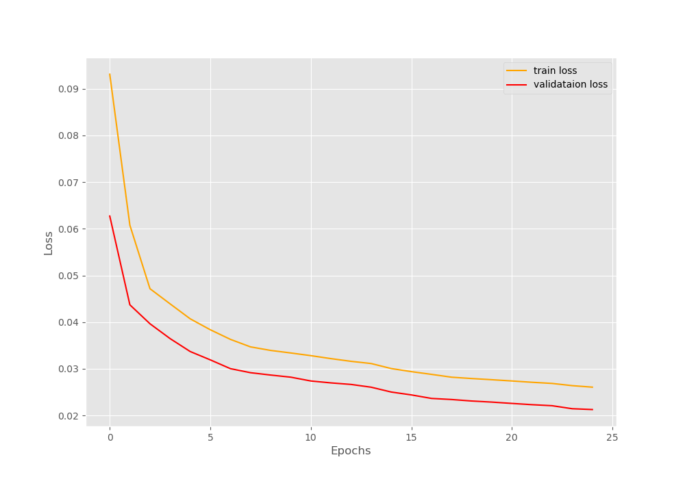
You can see that the training loss is higher than the validation loss until the end of the training. This because of the additional sparsity penalty that we are adding during training but not during validation.

Let’s take a look at the images that the autoencoder neural network has reconstructed during validation.

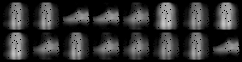
The above image shows that reconstructed image after the first epoch. We can see that the autoencoder finds it difficult to reconstruct the images due to the additional sparsity.

Now, let’s take look at a few other images.

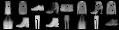
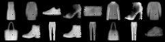
After the 10th iteration, the autoencoder model is able to reconstruct the images properly to some extent. By the last epoch, it has learned to reconstruct the images in a much better way.

Summary and Conclusion

The above results and images show that adding a sparsity penalty prevents an autoencoder neural network from just copying the inputs to the outputs. Instead, it learns many underlying features of the data.

In this tutorial you learned:

• The theory and mathematical concepts behind the KL divergence.
• How to train an autoencoder neural network with KL divergence using the PyTorch deep learning library.
• How adding a sparsity penalty helps an autoencoder model to learn the features of a data.

If you want to point out some discrepancies, then please leave your thoughts in the comment section. If you have any ideas or doubts, then you can use the comment section as well and I will try my best to address them.

You can contact me using the Contact section. You can also find me on LinkedIn, and Twitter.