Getting Started with Variational Autoencoders using PyTorch

Variational autoencoders (VAEs) are a group of generative models in the field of deep learning and neural networks. I say group because there are many types of VAEs. We will know about some of them shortly.

If you are new to autoencoders, then I recommend that you learn a bit about autoencoders before moving further. You can visit this link where you will find the basic and some advanced concepts about autoencoders. You will also get hands-on coding experience by going through these articles.

What will you learn in this tutorial?

• A brief recap about standard autoencoders and their limitations.
• About variational autoencoders and a short theory about their mathematics.
• Implementing a simple linear autoencoder on the MNIST digit dataset using PyTorch.

Note: This tutorial uses PyTorch. So it will be easier for you to grasp the coding concepts if you are familiar with PyTorch.

A Short Recap of Standard (Classical) Autoencoders

A standard autoencoder consists of an encoder and a decoder. Let the input data be X. The encoder produces the latent space vector z from X. Then the decoder tries to reconstruct the input data X from the latent vector z.

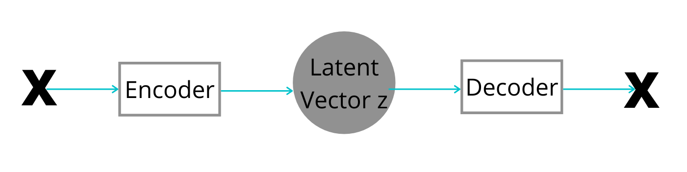
For example, let’s take the case of the MNIST digit dataset. Here, the input data X are all the digits in the dataset. The latent vector z consists of all the properties of the dataset that are not part of the original input data. Using these hidden (latent) vector properties, the decoder tries to reconstruct the original images again.

All of this sounds good, yet there are a few limitations to using standard autoencoders.

The Limitations of Standard Autoencoders

We now know that autoencoders are able to reconstruct the input data from the latent vectors. But the problem is that they can only reconstruct those types of images on which they are trained. In other words, they compress the data while producing the latent vector and try to replicate the output to the input.

Due to this, there are two major applications of standard autoencoder:

• Denoising of data, e.g. denoising images.
• Sparse reconstructions for dimensionality reduction.

Another limitation is that the latent space vectors are not continuous. This means that we can only replicate the output images to input images. But we cannot generate new images from the latent space vector. This is where variational autoencoders work much better than standard autoencoders.

Variational Autoencoders

The concept of variational autoencoders was introduced by Diederik P Kingma and Max Welling in their paper Auto-Encoding Variational Bayes.

Variational autoencoders or VAEs are really good at generating new images from the latent vector. Although, they also reconstruct images similar to the data they are trained on, but they can generate many variations of the images.

Moreover, the latent vector space of variational autoencoders is continous which helps them in generating new images.

In architecture, VAEs resemble a standard autoencoder. VAEs also consist of an encoder and a decoder. The major difference – the latent vector generated by VAEs is continuous which makes them a part of the generative neural network model family.

Types of Variational Autoencoders

VAEs also allow us to control or condition the outputs of the decoder to some extent. This conditioning of the decoder’s actions leads to the concept of Conditional Variational Autoencoders (CVAEs).

We can also have variational autoencoders that learn from latent vectors which have more disentanglement. As such, disentanglement can lead to learning a broader set of features from the input data to the latent vectors. This, we can control through a parameter called beta (\(\beta\)). Such VAEs are called \(\beta\)-VAEs.

However, in this tutorial, we will take a look at the simple VAE only. We will tackle other types of VAEs in future articles.

The Working of Variational Autoencoders

In this section we will go over the working of variational autoencoders. This section is going to be a bit technical. Our main focus is on the implementation of VAEs using coding. So, we will try to keep this section as short as possible.

I will highly recommend that you go through the original paper to get the most details about the mathematics behind VAEs.

The Problem

In the case of an autoencoder, we have \(z\) as the latent vector. We sample \(p_{\theta}(z)\) from \(z\). Then we sample the reconstruction given \(z\) as \(p_{\theta}(x|z)\). Here \(\theta\) are the learned parameters.

We want to maximize the log-likelihood of the data. The marginal likelihood is composed of a sum over the marginal likelihoods of individual datapoints. That is,

$$
logp_\theta(x^{(1)}, …, x^{(N)}) = \sum_{i=1}^{N}logp_\theta(x^{(i)})
$$

We can write this as:

$$
logp_\theta(x^{(i)}) = D_{KL}(q_{\phi}(z|x^{(i)}) || p_{\theta}(z|x^{(i)})) + \mathcal{L}(\theta, \phi;x^{(i)})
$$

In RHS, first, we have a KL divergence. This is the KL divergence between the approximated latent vector and the try latent vector of the encoder. Here, \(\phi\) are the approximated learned parameters. The second term is the variational lower bound.

The Variational Lower Bound

The variational lower bound is an important term. We can again write it as:

$$
\mathcal{L}(\theta, \phi;x^{(i)}) = -D_{KL}(q_{\phi}(z|x^{(i)}) || p_{\theta}(z)) + \mathbb{E}_{z{\tilde{}}q}[logp_{\theta}(x|z)]
$$

We need to maximize the variational lower bound by optimizing the parameters \(\phi\) and \(\theta\) of the neural network.

In simple words, on the RHS:

• We need to minimize the divergence between the estimated latent vector and the true latent vector.
• And we need to maximize the expectation of the reconstruction of data points from the latent vector.

Do not panic if the above formulae and concepts do not make much sense. You may have to go over the equations and the paper a few times to understand these. But it will be most helpful if you have a good grasp over the simple autoencoder concepts and the latent vector generation. Also, a bit of KL-Divergence knowledge will help. I highly recommend that you go through this article to get a better grasp of KL-Divergence.

There is just a bit more theory before we can move into the coding part. In fact, the last part of theory is one of the basic building blocks of implementation. It will also make the most sense in terms of understandability.

The Optimization Procedure

We need to maximize the \(\mathbb{E}{z{\tilde{}}q}[logp{\theta}(x|z)]\). Maximizing this means that the decoder is getting better at reconstruction. This means that we need to minimize reconstruction loss, which is \(\mathcal{L}_R\). This loss can be the Binary Cross-Entropy Loss (BCELoss).

Now, coming to minimizing \(D_{KL}(q_{\phi}(z|x^{(i)}) || p_{\theta}(z))\). This means, we need to maximize \(-D_{KL}(q_{\phi}(z|x^{(i)}) || p_{\theta}(z))\).

Rewriting it as:

$$
D_{KL}(q_{\phi}(z|x^{(i)}) || p_{\theta}(z)) = \frac{1}{2}\sum_{j=1}^{J}{(1+log(\sigma_j)^2-(\mu_j)^2-(\sigma_j)^2)}
$$

Here, \(\sigma_j\) is the standard deviation and \(\mu_j\) is the mean. For maximizing \(-D_{KL}\), we need \(\sigma_j\rightarrow1\) and \(\mu_j\rightarrow1\). Let’s call this loss as \(\mathcal{L}_{KL}\). And we sample \(\sigma\) and \(\mu\) from the encoder’s ouput.

So, the final VAE loss that we need to optimize is:

$$
\mathcal{L}_{VAE} = \mathcal{L}_R + \mathcal{L}_{KL}
$$

Finally, we need to sample from the input space using the following formula.

$$
Sample = \mu + \epsilon\sigma
$$

Here, \(\epsilon\sigma\) is element-wise multiplication. And the above formula is called the reparameterization trick in VAE. This perhaps is the most important part of a variational autoencoder. This makes it look like as if the sampling is coming from the input space instead of the latent vector space.

This marks the end of the mathematical details.

All of this will make more sense when we implement these in coding. And I again recommend going through the paper and my previous autoencoder blog posts.

The Directory Structure

We will use a very simple directory structure for this project.

├───input
│   └───data
├───outputs
└───src
    │   model.py
    │   train.py

The following are the descriptions of the different folders.

• input folder has a data subfolder where the MNIST dataset will get downloaded.
• outputs will contain the image reconstructions while training and validating the variational autoencoder model.
• The src folder contains two python scripts. One is model.py that contains the variational autoencoder model architecture. The other one is train.py that contains the code to train and validate the VAE on the MNIST dataset.

Implementing a Simple Variational Autoencder using PyTorch

Beginning from this section, we will focus on the coding part of this tutorial. I will be telling which python code will go into which file. We will start with building the VAE model.

Building our Linear VAE Model using PyTorch

The VAE model that we will build will consist of linear layers only. We will call our model LinearVAE(). All the code in this section will go into the model.py file.

Let’s import the following modules first.

import torch
import torch.nn as nn
import torch.nn.functional as F

The LinearVAE() Module

We will define the LinearVAE() module in a single block of code so as to maintain the continuity. After that we will get into the description part.

The following block of code defines the LinearVAE() model.

features = 16
# define a simple linear VAE
class LinearVAE(nn.Module):
    def __init__(self):
        super(LinearVAE, self).__init__()
 
        # encoder
        self.enc1 = nn.Linear(in_features=784, out_features=512)
        self.enc2 = nn.Linear(in_features=512, out_features=features*2)
 
        # decoder 
        self.dec1 = nn.Linear(in_features=features, out_features=512)
        self.dec2 = nn.Linear(in_features=512, out_features=784)

    def reparameterize(self, mu, log_var):
        """
        :param mu: mean from the encoder's latent space
        :param log_var: log variance from the encoder's latent space
        """
        std = torch.exp(0.5*log_var) # standard deviation
        eps = torch.randn_like(std) # `randn_like` as we need the same size
        sample = mu + (eps * std) # sampling as if coming from the input space
        return sample
 
    def forward(self, x):
        # encoding
        x = F.relu(self.enc1(x))
        x = self.enc2(x).view(-1, 2, features)

        # get `mu` and `log_var`
        mu = x[:, 0, :] # the first feature values as mean
        log_var = x[:, 1, :] # the other feature values as variance

        # get the latent vector through reparameterization
        z = self.reparameterize(mu, log_var)
 
        # decoding
        x = F.relu(self.dec1(z))
        reconstruction = torch.sigmoid(self.dec2(x))
        return reconstruction, mu, log_var

I know that this a bit different from a standard PyTorch model that contains only an __init__() and forward() function. But things will become very clear when we get into the description of the above code.

Description of the LinearVAE() Model

The features=16 is used in the output features for the encoder and the input features of the decoder.

First we have the __init__() function starting from line 4.

• We have a total of 4 linear layers here.
• The first two are the encoder layers. The self.enc1 has 784 in_features. This corresponds to the total number of pixels for image in the MNIST dataset (28x28x1). The out_features is 512.
• Simlarly, we have another encoder layer with 32 output features.
• The deocoder layers go in reverse order as that of the encoder layers. By this, finally we end up with 784 outputs features in self.dec2.

Then from line 15, we have the reparameterize() function.

• It has two parameters mu and log_var.
• mu is the mean that is coming from encoder’s latent space encoding.
• And log_var is the log variance that is coming from the encoder’s latent space.
• These are the same terms that we use in the Sample formula in one of the previous sections.
• At line 20, first, we calculate the standard deviation (std) using the log_var.
• Then at line 21, we calculate epsilon (eps) that we will use in the sample formula. We use torch.rand_like() so that dimensions will be same as std.
• At line 22, we calculate the sample using mu, eps, std. Then we return its value. Take a moment to go through the above equations and steps.

Starting from line 25, we have the forward() function.

• First, lines 27 and 28 pass the input through the VAE’s encoder layers. But note that line 28 does not give us the latent vector.
• Then we get mu and log_var at lines 31 and 32. These two have the same value as the encoder’s last layer output.
• At line 35, we get the latent vector z through the reparameterization trick using mu and log_var.
• From line 38 we have the decoding part. We pass the latent vector z through the first decoder layer. Then we get the reconstruction of the inputs by giving that output as input to the second decoder layer.
• Finally, at line 40 we return the reconstruction, mu, and log_var values.

This ends the model building part of our VAE implementation. Next, we will move into writing the training code.

Writing the Training Code for the VAE Implementation

In this section, we will write the code to train and validate the VAE model. The code in this section will go into the train.py file.

We will start with importing all the modules and libraries that we will need.

import torch
import torchvision
import torch.optim as optim
import argparse
import matplotlib
import torch.nn as nn
import matplotlib.pyplot as plt
import torchvision.transforms as transforms
import model

from tqdm import tqdm
from torchvision import datasets
from torch.utils.data import DataLoader
from torchvision.utils import save_image

matplotlib.style.use('ggplot')

• At line 9, we are importing model which contains our LinearVAE() model.
• Also, we are importing the save_image function from torchvision so that we able to save batches of images directly.

Construct the Argument Parser and Define the Learning Parameters

Now, we will define the argument parser to parse the command line arguments. We will provide the number of epochs to train for as the argument while executing the file from the command line. The following block of code constructs the argument parser.

# construct the argument parser and parser the arguments
parser = argparse.ArgumentParser()
parser.add_argument('-e', '--epochs', default=10, type=int, 
                    help='number of epochs to train the VAE for')
args = vars(parser.parse_args())

Next, we will define the learning parameters for training our model.

# leanring parameters
epochs = args['epochs']
batch_size = 64
lr = 0.0001
device = torch.device('cuda' if torch.cuda.is_available() else 'cpu')

• At line 2, we get the number of epochs from the argument parser.
• Then we define a batch size of 64 at line 3.
• We will use a learning rate of 0.0001.
• Finally, at line 5, we define the computation device, which is either the CPU or the GPU.

Preparing the MNIST Dataset

We will start with defining the transforms. For the transforms, we will only convert the data into torch tensors. We will not augment or rotate the data in any way. Either rotating or horizontally flipping the digit images can compromise the orientation information of the data.

# transforms
transform = transforms.Compose([
    transforms.ToTensor(),
])

Now, we will get the test data and validation data using the datasets module from torchvision. If the data is not already present, then it will be downloaded to the respective folder.

# train and validation data
train_data = datasets.MNIST(
    root='../input/data',
    train=True,
    download=True,
    transform=transform
)
val_data = datasets.MNIST(
    root='../input/data',
    train=False,
    download=True,
    transform=transform
)

After this, we have to define the train and validation data loaders. We can easily do that using the DataLoader module from PyTorch.

# training and validation data loaders
train_loader = DataLoader(
    train_data,
    batch_size=batch_size,
    shuffle=True
)
val_loader = DataLoader(
    val_data,
    batch_size=batch_size,
    shuffle=False
)

This is all the data preparation that we need.

Initializing the Model, the Optimizer, and the Loss Function

We will start initialing the model and loading it onto the computation device. Then we will define the optimizer and the loss function.

model = model.LinearVAE().to(device)
optimizer = optim.Adam(model.parameters(), lr=lr)
criterion = nn.BCELoss(reduction='sum')

We are using the Adam optimizer for training. The loss function here is the Binary Cross Entropy loss. We will use it to calculate the reconstruction loss. Basically, it will calculate the loss between the actual input data points and the reconstructed data points. This is only part of the total loss. We will also have to calculate the KL divergence as well.

Note that we are using reduction='sum' for the BCELoss(). If you read the PyTorch documentations, then this is specifically for the case of autoencoders only.

The Final Loss Function

Here, we will write the function to calculate the total loss while training the autoencoder model. Remember that it is going to be the addition of the KL Divergence loss and the reconstruction loss.

def final_loss(bce_loss, mu, logvar):
    """
    This function will add the reconstruction loss (BCELoss) and the 
    KL-Divergence.
    KL-Divergence = 0.5 * sum(1 + log(sigma^2) - mu^2 - sigma^2)

    :param bce_loss: recontruction loss
    :param mu: the mean from the latent vector
    :param logvar: log variance from the latent vector
    """
    BCE = bce_loss 
    KLD = -0.5 * torch.sum(1 + logvar - mu.pow(2) - logvar.exp())

    return BCE + KLD

final_loss() function has three parameters. The bce_loss is the Binary Cross Entropy reconstruction loss. The mu and log_var are the values that we get from the autoencoder model.

• First, we initialize the Binary Cross Entropy loss at line 11.
• At line 12, we calculate the KL divergence using the mu and log_var values.
• Finally, we return the total loss at line 14.

The Training Function

We will define the training function here. We will call it as fit().

def fit(model, dataloader):
    model.train()
    running_loss = 0.0
    for i, data in tqdm(enumerate(dataloader), total=int(len(train_data)/dataloader.batch_size)):
        data, _ = data
        data = data.to(device)
        data = data.view(data.size(0), -1)
        optimizer.zero_grad()
        reconstruction, mu, logvar = model(data)
        bce_loss = criterion(reconstruction, data)
        loss = final_loss(bce_loss, mu, logvar)
        running_loss += loss.item()
        loss.backward()
        optimizer.step()

    train_loss = running_loss/len(dataloader.dataset)
    return train_loss

The fit() function accepts two parameters, the model and the train_loader as dataloader. At line 2, first, we get into training mode.

• At line 3, we initialize running_loss to keep track of the batch-wise loss values.
• Line 7, flattens the input data as we are going to feed it into a linear layer.
• At line 9, we get the reconstruction, mu, and log_var.
• Line 10 calculates the reconstruction loss using the reconstructed data and the original input data.
• At line 11, we calculate the total loss using the total_loss function.
• We calculate the batch loss at line 12. Then we backpropagate the gradients and update the parameters at lines 13 and 14 respectively.
• Finally, we calculate the total loss for the epoch (train_loss) and return its value.

The Validation Function

The validation function will be very similar to the training function with a few minor changes. We will call the function as validate().

def validate(model, dataloader):
    model.eval()
    running_loss = 0.0
    with torch.no_grad():
        for i, data in tqdm(enumerate(dataloader), total=int(len(val_data)/dataloader.batch_size)):
            data, _ = data
            data = data.to(device)
            data = data.view(data.size(0), -1)
            reconstruction, mu, logvar = model(data)
            bce_loss = criterion(reconstruction, data)
            loss = final_loss(bce_loss, mu, logvar)
            running_loss += loss.item()
        
            # save the last batch input and output of every epoch
            if i == int(len(val_data)/dataloader.batch_size) - 1:
                num_rows = 8
                both = torch.cat((data.view(batch_size, 1, 28, 28)[:8], 
                                  reconstruction.view(batch_size, 1, 28, 28)[:8]))
                save_image(both.cpu(), f"../outputs/output{epoch}.png", nrow=num_rows)

    val_loss = running_loss/len(dataloader.dataset)
    return val_loss

First, we get the model into evaluation mode using model.eval(). And everything takes place within the with torch.no_grad() block as we do not need the gradients during validation.

• Just like the training function, we calculate the losses at lines 11 and 12.
• At line 15, we check if we are at the last batch of every epoch. If we are at the last batch, then we concatenate the first eight images of the input data and the first eight images of the reconstructed data. Then we save the image batch using the save_image function. This will help us easily compare the real data to the reconstructed data.
• Then at line 21, we calculate the total validation loss and return the value.

Executing the fit() and validate() Functions

This is the last part of this training script. We need to train and validate our VAE model for the specified number of epochs.

train_loss = []
val_loss = []
for epoch in range(epochs):
    print(f"Epoch {epoch+1} of {epochs}")
    train_epoch_loss = fit(model, train_loader)
    val_epoch_loss = validate(model, val_loader)
    train_loss.append(train_epoch_loss)
    val_loss.append(val_epoch_loss)
    print(f"Train Loss: {train_epoch_loss:.4f}")
    print(f"Val Loss: {val_epoch_loss:.4f}")

• We will use the train_loss and val_loss (lines 1 and 2) lists to store the train and validation losses respectively.
• Then we use a for loop to train the model for the number of epochs as specified in the command line argument.

This all that we need for the training script. Next, we will execute the code and analyze the outputs.

Executing the train.py Script

We have all the code ready to train our VAE on the MNIST dataset. Now, we just need to execute the train.py script.

You will need to open up the terminal and head over to the src folder in the terminal. From there you can execute the train.py script for 20 epochs.

python train.py --epochs 20

Your training will take less time if you run it on a GPU. The following is the truncated output from the command line.

Epoch 1 of 20
938it [00:12, 72.58it/s]
157it [00:01, 103.02it/s]
Train Loss: 213.8055
Val Loss: 163.1456
Epoch 2 of 20
938it [00:12, 73.58it/s]
157it [00:01, 103.98it/s]
Train Loss: 151.8054
Val Loss: 139.9007
...
Epoch 19 of 20
938it [00:12, 73.90it/s]
157it [00:01, 98.42it/s]
Train Loss: 109.0154
Val Loss: 108.3255
Epoch 20 of 20
938it [00:12, 73.25it/s]
157it [00:01, 97.43it/s]
Train Loss: 108.7223
Val Loss: 107.8552

After each validation epoch, we are saving the original input data and the reconstructed images to the disk. We will analyze those in the next section.

Analyzing the Image Reconstructions

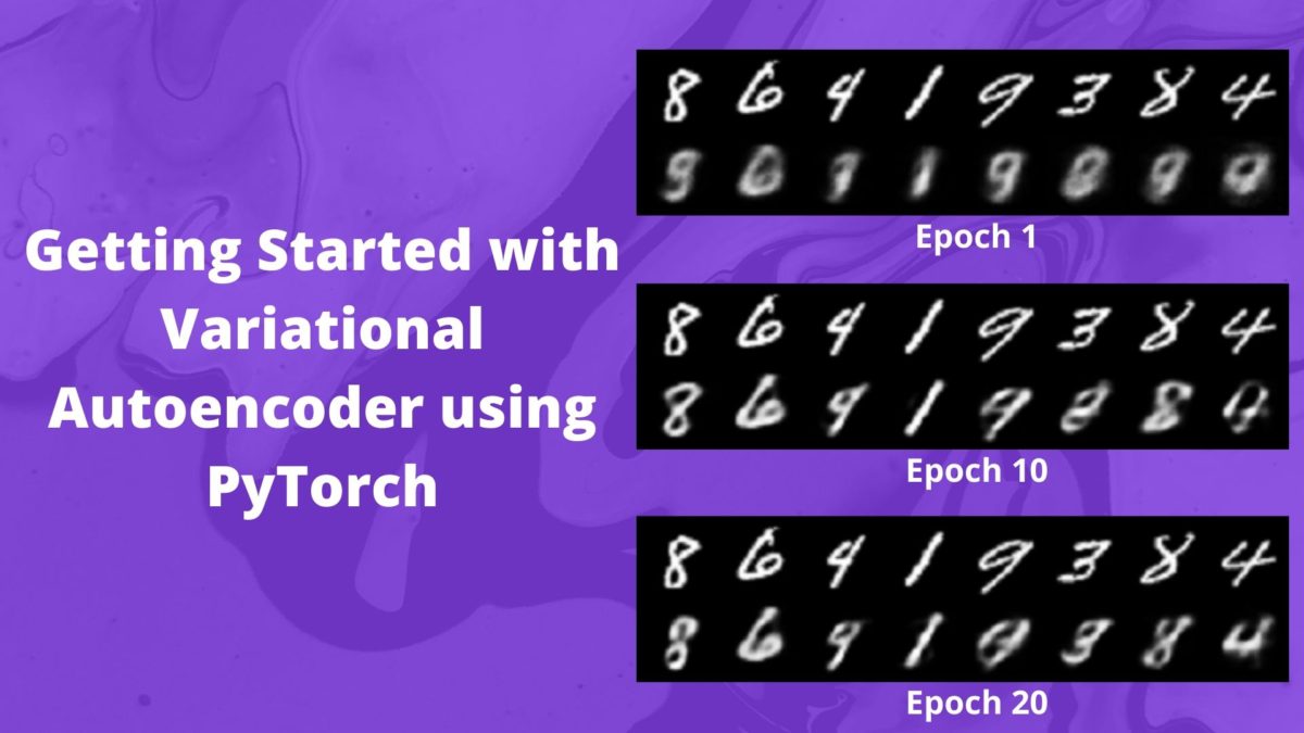
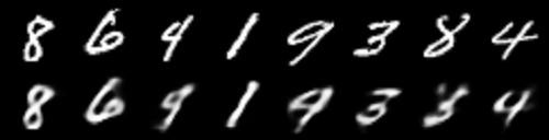
Let’s start with very first output. That is, the output from the first validation epoch.

The reconstructions from the first epoch are a bit blurry. Moreover, the VAE model has reconstructed the digit 8 as 9 in all cases. And it has reconstructed the digit 4 as 0. This is expected as VAE tries to reconstruct the original images from a continuous vector space. So, most probably it will generate an image closer to something else when it is not very sure.

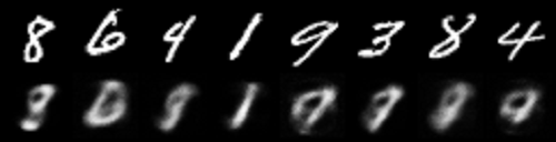
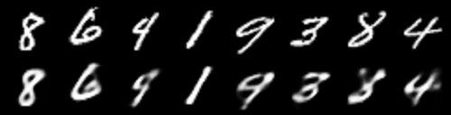
Now, let’s see the reconstructions after 10 epochs.

In figure 4, we can see that the reconstructions are much better and clearer. But still, the digit 4 (third from the left) is being reconstructed as a 9. And the digit 9 (fifth from the left) is being reconstructed as a 0.

Let’s hope that the outputs are even better in the last epoch (epoch 20).

All the images except the 3 (third from right) are properly reconstructed. This digit 3 is being reconstructed as an eight. It is very clear that training for more epochs will yield even better results.

Summary and Conclusion

In this tutorial, you learned about the concept of variational autoencoders in deep learning. You also had hands-on experience and implemented a simple linear variational autoencoder model to reconstruct the digit MNIST images. I hope that you learned a lot from this tutorial.

If you have any thoughts, suggestions, or doubts, then please leave them in the comment section. I will surely address them.

You can contact me using the Contact section. You can also find me on LinkedIn, and Twitter.