Generating MNIST Digit Images using Vanilla GAN with PyTorch

In this tutorial, we will generate the digit images from the MNIST digit dataset using Vanilla GAN. We will use the PyTorch deep learning framework to build and train the Generative Adversarial network.

If you are new to Generative Adversarial Networks in deep learning, then I would highly recommend you go through the basics first. You may read my previous article (Introduction to Generative Adversarial Networks). By going through that article you will:

• Learn the basic architecture of generative adversarial networks.
• Get to learn about the training of the generator and the discriminator.
• Know how the loss function works for the generator and the discriminator in a GAN.
• Know about the different architectures and applications of GANs.

After going through the introductory article on GANs, you will find it much easier to follow through this coding tutorial.

What Will You Learn in This Tutorial?

Before moving further, let’s discuss what you will learn after going through this tutorial. You will:

• Get to know how to build a generative adversarial network (Vanilla GAN) to generate the MNIST digit dataset images.
• Learn about the training of generator and discriminator through coding using the PyTorch deep learning framework. We will build the Vanilla GAN architecture using Linear neural network layers.
• Know the steps to train a generative adversarial network in a well-formed manner.
• Know how to save the generated images to effectively analyze the results.
• BONUS – a Colab link at the end containing the code for a different dataset.

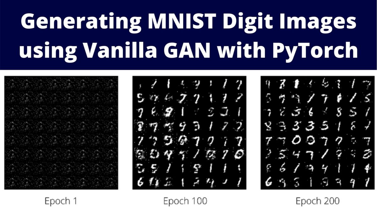
You may have a look at the following image. You will get a feel of how interesting this is going to be if you stick till the end.

The image on the right side is generated by the generator after training for one epoch. Clearly, nothing is here except random noise. Now take a look a the image on the right side. This image is generated by the generator after training for 200 epochs. Now that looks promising and a lot better than the adjacent one. Further in this tutorial, we will learn, step-by-step, how to get from the left image to the right image.

How to Train a Vanilla GAN using PyTorch?

In this section, we will take a look at the steps for training a generative adversarial network. In my opinion, this is a very important part before we move into the coding part. This will help us to articulate how we should write the code and what the flow of different components in the code should be.

I hope that after going through the steps of training a GAN, it will be much easier for you to absorb the concepts while coding.

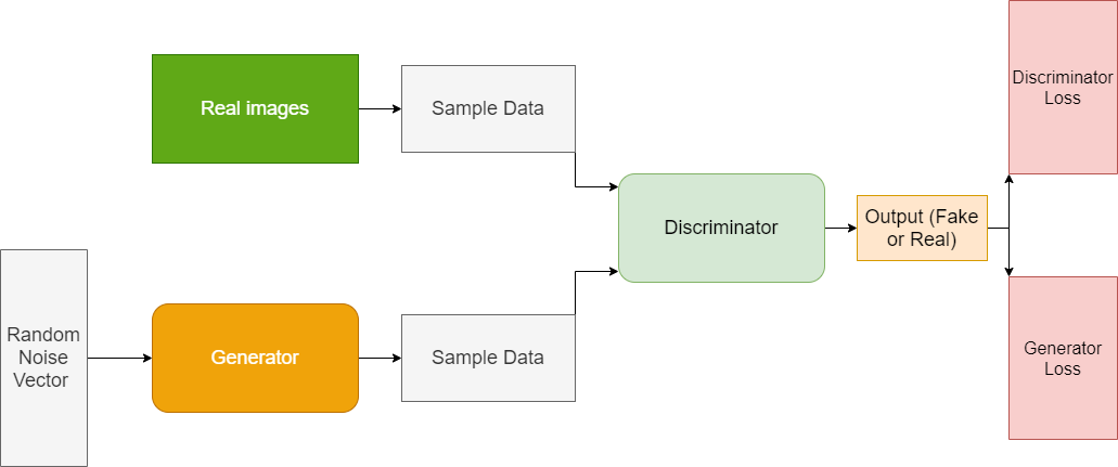
We know that while training a GAN, we need to train two neural networks simultaneously. One is the discriminator and the other is the generator. To get the desired and effective results, the sequence in this training procedure is very important.

Training the Discriminator

• First, we get the real data and the real labels (real labels are all 1s). The length of the real label should be equal to the batch size.
• Then we do a forward pass by feeding the real data to the discriminator neural network. This gives us the real outputs from the real data.
• Calculate the discriminator loss for the real outputs and labels and backpropagate it.
• Get the fake data using the noise vector and do a forward pass through the generator. Get fake labels as well.
• Using the fake data, do a forward pass through the discriminator. Calculate the loss using the fake data outputs and the fake labels. Backpropagate the fake data loss. Then calculate the total discriminator loss by adding real data loss and fake data loss.
• Update the discriminator optimizer parameters.

Training the Generator

• For the generator training, first, get the fake data by doing a forward pass through the generator. Get the real labels (all 1s).
• Then do a forward pass through the discriminator using the fake data and the labels.
• Calculate the loss and backpropagate them.
• But this time, update the generator optimizer parameters.

The last few steps may seem a bit confusing. Especially, “why do we need to forward pass the fake data through the discriminator to update the generator parameters?” This is because, the discriminator would tell how well the generator did while generating the fake data. Do take some time to think about this point. All of this will become even clearer while coding. So, hang on for a bit.

The Project Structure

We will use the following project structure to manage everything while building our Vanilla GAN in PyTorch.

├───input
├───outputs
└───src
        vanilla_gan.py

• The MNIST dataset will be downloaded into the input folder. We will use the datasets module from torchvision to download the dataset.
• The outputs folder will contain all the outputs while training the GAN. This includes the images that are generated by the generator, the loss plots, and the final model as well.
• Inside the src folder, we have the vanilla_gan.py script. We will write all the code training our GAN inside this python file.

And obviously, we will be using the PyTorch deep learning framework in this article. So, you may go ahead and install it if you do not have it already.

Training Vanilla GAN to Generate MNIST Digits using PyTorch

From this section onward, we will be writing the code to build and train our vanilla GAN model on the MNIST Digit dataset. Hopefully, by the end of this tutorial, we will be able to generate images of digits by using the trained generator model.

So, let’s start coding our way through this tutorial. We will write all the code inside the vanilla_gan.py file.

Importing All the Required Modules and Libraries

The first step is to import all the modules and libraries that we will need, of course.

import torch
import torch.nn as nn
import torchvision.transforms as transforms
import torch.optim as optim
import torchvision.datasets as datasets
import imageio
import numpy as np
import matplotlib

from torchvision.utils import make_grid, save_image
from torch.utils.data import DataLoader
from matplotlib import pyplot as plt
from tqdm import tqdm

matplotlib.style.use('ggplot')

Among all the known modules, we are also importing the make_grid and save_image functions from torchvision.utils. These two functions will help us save PyTorch tensor images in a very effective and easy manner without much hassle.

Defining the Learning Parameters

This is an important section where we will define the learning parameters for our generative adversarial network. Let’s define the learning parameters first, then we will get down to the explanation.

# learning parameters
batch_size = 512
epochs = 200
sample_size = 64 # fixed sample size
nz = 128 # latent vector size
k = 1 # number of steps to apply to the discriminator
device = torch.device('cuda' if torch.cuda.is_available() else 'cpu')

• First, we have the batch_size which is pretty common. I have used a batch size of 512. As the MNIST images are very small (28×28 greyscale images), using a larger batch size is not a problem. You may use a smaller batch size if your run into OOM (Out Of Memory error). But I recommend using as large a batch size as your GPU can handle for training GANs. GAN training can be much faster while using larger batch sizes.
• Then we have the number of epochs. We will train our GAN for 200 epochs. GAN training takes a lot of iterations. And for converging a vanilla GAN, it is not too out of place to train for 200 or even 300 epochs.
• The next one is the sample_size parameter which is an important one. We will be sampling a fixed-size noise vector that we will feed into our generator. Using the noise vector, the generator will generate fake images.
• Then we have the nz parameter. This is the latent vector or the noise vector size. The input feature size for the generator is going to be the same as this latent vector size. It is always better to define these in one place and use the variable names. Else, we may run into a lot of errors if we use the numerical values directly.
• k is a hyperparameter that indicates the number of steps to apply to the discriminator. If you want to know more, you can check Algorithm 1 in the paper, Generative Adversarial Nets. We will keep the value of k as 1 as this is the least expensive training option.
• Finally, we define the computation device. I recommend using a GPU for GAN training as it takes a lot of time. If you do not have a GPU in your local machine, then you should use Google Colab or Kaggle Kernel.

These are the learning parameters that we need. Now, let’s move on to preparing out dataset.

Preparing the Dataset

We will define the dataset transforms first. The following block of code defines the image transforms that we need for the MNIST dataset.

transform = transforms.Compose([
                                transforms.ToTensor(),
                                transforms.Normalize((0.5,),(0.5,)),
])

to_pil_image = transforms.ToPILImage()

• At line 1, we define transform which will convert the image to tensors and normalizes them as well.
• At line 6, we define to_pil_image. This will convert the images to the PIL image format. This is required when we want to save the images that are generated by the generator as a .gif file. Before saving them, we need to convert them into the PIL image format. We will combine all the generated images from the 200 epochs and save the reconstructions as a .gif file that we can analyze after training.

The next block of code defines the training dataset and training data loader. We will download the MNIST dataset using the dataset module from torchvision.

train_data = datasets.MNIST(
    root='../input/data',
    train=True,
    download=True,
    transform=transform
)
train_loader = DataLoader(train_data, batch_size=batch_size, shuffle=True)

This is all that we need regarding the dataset. In the following two sections, we will define the generator and the discriminator network of Vanilla GAN.

The Generator Neural Network

Let’s start with building the generator neural network.

It is going to be a very simple network with Linear layers, and LeakyReLU activations in-between.

class Generator(nn.Module):
    def __init__(self, nz):
        super(Generator, self).__init__()
        self.nz = nz
        self.main = nn.Sequential(
            nn.Linear(self.nz, 256),
            nn.LeakyReLU(0.2),

            nn.Linear(256, 512),
            nn.LeakyReLU(0.2),

            nn.Linear(512, 1024),
            nn.LeakyReLU(0.2),

            nn.Linear(1024, 784),
            nn.Tanh(),
        )

    def forward(self, x):
        return self.main(x).view(-1, 1, 28, 28)

We have the __init__() function starting from line 2. It accepts the nz parameter which is going to be the number of input features for the first linear layer of the generator network.

• We are using the Sequential container to build the neural network.
• The first linear layer (line 6) has in_features equal to nz, that is 128. The out_features is 256. Then we have a LeakyReLU activation with negative slope of 0.2.
• We have a total of four Linear layers and three LearkyReLU activations. The last layer’s activation is Tanh.

Then we have the forward() function starting from line 19. It does a forward pass of the batch of images through the neural network. It returns the outputs after reshaping them into batch_size x 1 x 28 x 28.

The Discriminator Neural Network

Here we will define the discriminator neural network.

Remember that the discriminator is a binary classifier. Therefore, we will have to take that into consideration while building the discriminator neural network.

class Discriminator(nn.Module):
    def __init__(self):
        super(Discriminator, self).__init__()
        self.n_input = 784
        self.main = nn.Sequential(
            nn.Linear(self.n_input, 1024),
            nn.LeakyReLU(0.2),
            nn.Dropout(0.3),

            nn.Linear(1024, 512),
            nn.LeakyReLU(0.2),
            nn.Dropout(0.3),

            nn.Linear(512, 256),
            nn.LeakyReLU(0.2),
            nn.Dropout(0.3),

            nn.Linear(256, 1),
            nn.Sigmoid(),
        )

    def forward(self, x):
        x = x.view(-1, 784)
        return self.main(x)

Starting from line 2, we have the __init__() function.

• At line 4, we define self.n_input = 784 which is the flattened size of the MNIST images (28×28). This is going to be the in_feature for the first layer.
• Starting from line 5, we define the discriminator network using the Sequential container.
• Here, we use Linear layers and LeakyReLU activations as well. Along with that, we use Dropout with rate of 0.3 after the first three Linear layers.
• We are using the Sigmoid activation after the last Linear layer (lines 18 and 19).
• The forward() function (line 22) makes a forward pass of the data through the discriminator network. It returns the binary classification of whether an image is fake or real (0 or 1) (line 24).

Initialize the Neural Networks and Define the Optimizers

Before moving further, we need to initialize the generator and discriminator neural networks.

generator = Generator(nz).to(device)
discriminator = Discriminator().to(device)

print('##### GENERATOR #####')
print(generator)
print('######################')

print('\n##### DISCRIMINATOR #####')
print(discriminator)
print('######################')

Note that we are passing the nz (the noise vector size) as an argument while initializing the generator network.

The next step is to define the optimizers. We need to update the generator and discriminator parameters differently. Therefore, we will initialize the Adam optimizer twice. Once for the generator network and again for the discriminator network.

# optimizers
optim_g = optim.Adam(generator.parameters(), lr=0.0002)
optim_d = optim.Adam(discriminator.parameters(), lr=0.0002)

Both of them are Adam optimizers with learning rate of 0.0002.

We will also need to define the loss function here. We will use the Binary Cross Entropy Loss Function for this problem.

# loss function
criterion = nn.BCELoss()

While training the generator and the discriminator, we need to store the epoch-wise loss values for both the networks. We will define two lists for this task. We will also need to store the images that are generated by the generator after each epoch. For that also, we will use a list.

losses_g = [] # to store generator loss after each epoch
losses_d = [] # to store discriminator loss after each epoch
images = [] # to store images generatd by the generator

In the next section, we will define some utility functions that will make some of the work easier for us along the way.

Defining Some Utility Functions

For training the GAN in this tutorial, we need the real image data and the fake image data from the generator. To calculate the loss, we also need real labels and the fake labels. Those will have to be tensors whose size should be equal to the batch size.

Let’s define two functions, which will create tensors of 1s (ones) and 0s (zeros) for us whose size will be equal to the batch size.

# to create real labels (1s)
def label_real(size):
    data = torch.ones(size, 1)
    return data.to(device)

# to create fake labels (0s)
def label_fake(size):
    data = torch.zeros(size, 1)
    return data.to(device)

For generating fake images, we need to provide the generator with a noise vector. The size of the noise vector should be equal to nz (128) that we have defined earlier. To create this noise vector, we can define a function called create_noise().

# function to create the noise vector
def create_noise(sample_size, nz):
    return torch.randn(sample_size, nz).to(device)

The function create_noise() accepts two parameters, sample_size and nz. It will return a vector of random noise that we will feed into our generator to create the fake images.

There is one final utility function. We need to save the images generated by the generator after each epoch. Now, they are torch tensors. To save those easily, we can define a function which takes those batch of images and saves them in a grid-like structure.

# to save the images generated by the generator
def save_generator_image(image, path):
    save_image(image, path)

The above are all the utility functions that we need. In the following sections, we will define functions to train the generator and discriminator networks.

Function to Train the Discriminator

First, we will write the function to train the discriminator, then we will move into the generator part.

Let’s write the code first, then we will move onto the explanation part.

# function to train the discriminator network
def train_discriminator(optimizer, data_real, data_fake):
    b_size = data_real.size(0)
    real_label = label_real(b_size)
    fake_label = label_fake(b_size)

    optimizer.zero_grad()

    output_real = discriminator(data_real)
    loss_real = criterion(output_real, real_label)

    output_fake = discriminator(data_fake)
    loss_fake = criterion(output_fake, fake_label)


    loss_real.backward()
    loss_fake.backward()
    optimizer.step()

    return loss_real + loss_fake

• At line 3, we get the batch size of the data. Then we use the batch size to create the fake and real labels at lines 4 and 5.
• Before doing any training, we first set the gradients to zero at line 7.
• At line 9, we get the output_real by doing a forward pass of the real data (data_real) through the discriminator. Line 10 calculates the loss for the real outputs and the real labels.
• Similarly, at line 12, we get fake outputs using fake data. And line 13, calculates the loss for the fake outputs and the fake labels.
• Lines 16 to 18 backpropagate the gradients for the fake and the real loss and update the parameters as well.
• Finally, at line 20, we return the total loss for the discriminator network.

I hope that the above steps make sense. If you are feeling confused, then please spend some time to analyze the code before moving further.

Function to Train the Generator

Now, we will write the code to train the generator. This is going to a bit simpler than the discriminator coding.

# function to train the generator network
def train_generator(optimizer, data_fake):
    b_size = data_fake.size(0)
    real_label = label_real(b_size)

    optimizer.zero_grad()

    output = discriminator(data_fake)
    loss = criterion(output, real_label)

    loss.backward()
    optimizer.step()

    return loss

• First, we get the batch size at line 3 and then create the real labels at line 4. Remember that the fake data is actually real for the generator. Therefore, we are using real labels (ones) for training the generator network.
• At line 6, we set the gradients to zero.
• The next step is a bit important. At line 8, we pass the fake data through the discriminator and get the outputs. Then at line 9, we calculate the loss using the outputs and the real labels.
• Remember that the generator only generates fake data. And it improves after each iteration by taking in the feedback from the discriminator.
• At line 11, we backpropagate the gradients.
• Now, at line 12, we update the generator parameters and not the discriminator parameters. Because in this step, we want the generator to learn, not the discriminator. The optimizer parameter in the function definition is the optim_g that we will pass as the argument while calling the function.

Training the Vanilla GAN

In this section, we will write the code to train the GAN for 200 epochs.

First, let’s create the noise vector that we will need to generate the fake data using the generator network.

# create the noise vector
noise = create_noise(sample_size, nz)

It is also a good idea to switch both the networks to training mode before moving ahead.

generator.train()
discriminator.train()

The Training Loop

We will use a simple for loop for training our generator and discriminator networks for 200 epochs. We will write the code in one whole block to maintain the continuity.

for epoch in range(epochs):
    loss_g = 0.0
    loss_d = 0.0
    for bi, data in tqdm(enumerate(train_loader), total=int(len(train_data)/train_loader.batch_size)):
        image, _ = data
        image = image.to(device)
        b_size = len(image)
        # run the discriminator for k number of steps
        for step in range(k):
            data_fake = generator(create_noise(b_size, nz)).detach()
            data_real = image
            # train the discriminator network
            loss_d += train_discriminator(optim_d, data_real, data_fake)
        data_fake = generator(create_noise(b_size, nz))
        # train the generator network
        loss_g += train_generator(optim_g, data_fake)

    # create the final fake image for the epoch
    generated_img = generator(noise).cpu().detach()
    # make the images as grid
    generated_img = make_grid(generated_img)
    # save the generated torch tensor models to disk
    save_generator_image(generated_img, f"../outputs/gen_img{epoch}.png")
    images.append(generated_img)
    epoch_loss_g = loss_g / bi # total generator loss for the epoch
    epoch_loss_d = loss_d / bi # total discriminator loss for the epoch
    losses_g.append(epoch_loss_g)
    losses_d.append(epoch_loss_d)
    
    print(f"Epoch {epoch} of {epochs}")
    print(f"Generator loss: {epoch_loss_g:.8f}, Discriminator loss: {epoch_loss_d:.8f}")

Explanation of the Training Loop

• At lines 2 and 3, we define loss_g and loss_d to keep track of the batch-wise loss values for the discriminator and the generator.
• Starting from line 4, we iterate through the batches. We only need the image data. Therefore, we get the images only at line 5 and load them to the computation device at line 6. Line 7 calculates the batch size.
• Starting from line 9 till 13, we run the discriminator for k number of steps. And remember that for our purpose we have defined k = 1. This is the least expensive option as this will train one step of the discriminator and one step of the generator. You can play around with the value of k. But remember that the computation time will also increase with an increase in the value of k.
• Also, note that we are passing the discriminator optimizer while calling train_discriminator() at line 13.
• At line 14, we again create a new noise vector. This we pass as an argument along with the generator optimizer while calling train_generator().
• At line 19, we create the final fake images for the current epoch and load them onto the CPU so that we can save them to the disk. Line 21 makes a grid of those images.
• Line 23 saves the generated images to disk. And line 24 appends those images to the images list.
• Finally, from line 25 to 31, we calculate the epoch-wise loss of the generator and the discriminator and print those loss values.

The Final Steps

These are some of the final coding steps that we need to carry. Let’s start with saving the trained generator model to disk.

print('DONE TRAINING')
torch.save(generator.state_dict(), '../outputs/generator.pth')

Next, we will save all the images generated by the generator as a Giphy file. This will help us to analyze the results better and also it is quite fun to see the images being generated as video after each iteration.

# save the generated images as GIF file
imgs = [np.array(to_pil_image(img)) for img in images]
imageio.mimsave('../outputs/generator_images.gif', imgs)

Finally, we will save the generator and discriminator loss plots to the disk.

# plot and save the generator and discriminator loss
plt.figure()
plt.plot(losses_g, label='Generator loss')
plt.plot(losses_d, label='Discriminator Loss')
plt.legend()
plt.savefig('../outputs/loss.png')

This marks the end of writing the code for training our GAN on the MNIST images. Now it is time to execute the python file.

Execute the vanilla_gan.py File

Open up your terminal and cd into the src folder in the project directory. Then type the following command to execute the vanilla_gan.py file.

python vanilla_gan.py

I am showing only a part of the output below.

##### GENERATOR #####
Generator(
  (main): Sequential(
    (0): Linear(in_features=128, out_features=256, bias=True)
    (1): LeakyReLU(negative_slope=0.2)
    (2): Linear(in_features=256, out_features=512, bias=True)
    (3): LeakyReLU(negative_slope=0.2)
    (4): Linear(in_features=512, out_features=1024, bias=True)
    (5): LeakyReLU(negative_slope=0.2)
    (6): Linear(in_features=1024, out_features=784, bias=True)
    (7): Tanh()
  )
)
...
118it [00:11, 10.33it/s]
Epoch 0 of 200
Generator loss: 1.35006404, Discriminator loss: 0.93073928
118it [00:11, 10.53it/s]
Epoch 1 of 200
Generator loss: 2.95911145, Discriminator loss: 1.26289415
...
Epoch 198 of 200
Generator loss: 1.24842966, Discriminator loss: 1.08716691
118it [00:12,  9.47it/s]
Epoch 199 of 200
Generator loss: 1.30664957, Discriminator loss: 1.07282817
DONE TRAINING

As a matter of fact, there is not much that we can infer from the outputs on the screen. Let’s hope the loss plots and the generated images provide us with a better analysis.

Analyzing the Loss Plots and the Images Generated by the Vanilla GAN

Let’s look at the loss plot first.

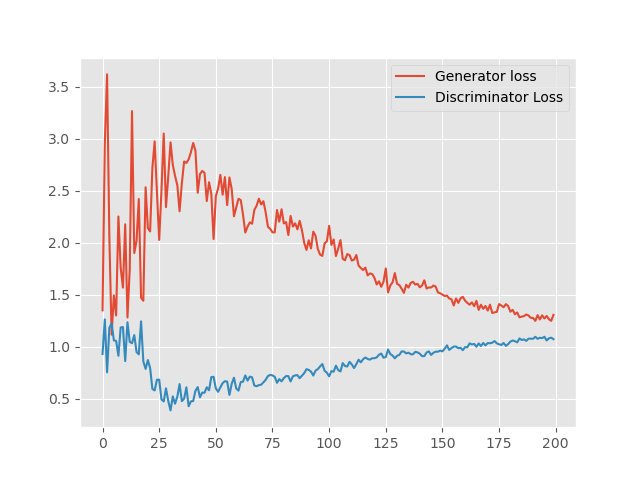
We can see that for the first few epochs the loss values of the generator are increasing and the discriminator losses are decreasing. This is because during the initial phases the generator does not create any good fake images. The discriminator easily classifies between the real images and the fake images. As the training progresses, the generator slowly starts to generate more believable images. At this time, the discriminator also starts to classify some of the fake images as real. Therefore, the generator loss begins to decrease and the discriminator loss begins to increase.

Also, we can clearly see that training for more epochs will surely help.

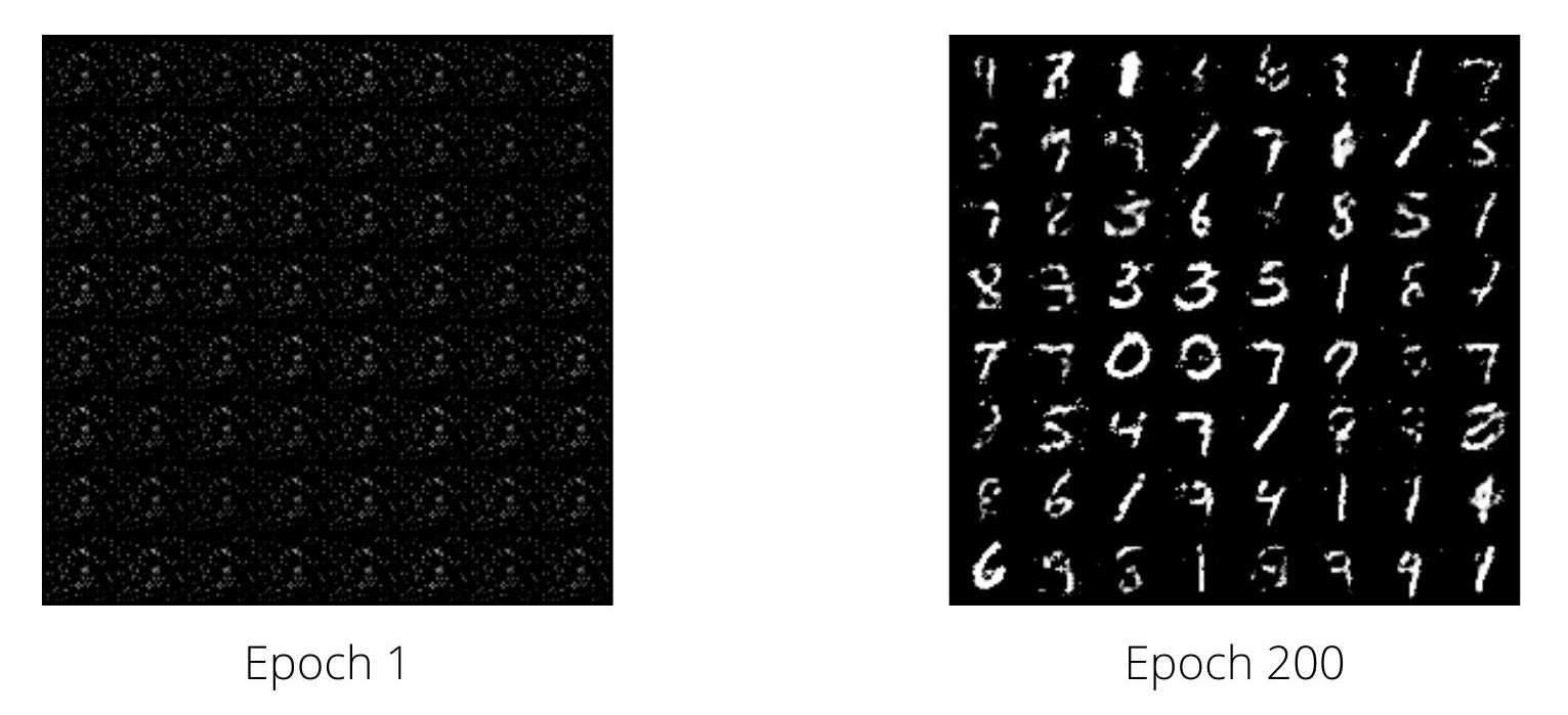
Now, let’s look at the generated images.

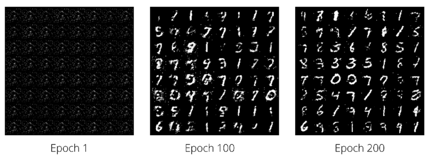
In figure 4, the first image shows the image generated by the generator after the first epoch. It is quite clear that those are nothing except noise. The second image is generated after training for 100 epochs. This looks a lot more promising than the previous one. Although we can still see some noisy pixels around the digits. The last one is after 200 epochs. Here, the digits are much more clearer. The noise is also less. But it is by no means perfect. There is a lot of room for improvement here.

For the final part, let’s see the Giphy that we saved to the disk.

The above clip shows how the generator generates the images after each epoch. We can see the improvement in the images after each epoch very clearly.

Bonus Colab Notebook

I am also attaching the link to a Google Colab notebook which trains a Vanilla GAN network on the Fashion MNIST dataset. Do take a look at it and try to tweak the code and different parameters. You will get to learn a lot that way. Find the notebook here.

Summary and Conclusion

In this tutorial, you learned how to write the code to build a vanilla GAN using linear layers in PyTorch. You also learned how to train the GAN on MNIST images. There are many more types of GAN architectures that we will be covering in future articles. Some of them include DCGAN (Deep Convolution GAN) and the CGAN (Conditional GAN).

I hope that you learned new things from this tutorial. If you have any doubts, thoughts, or suggestions, then leave them in the comment section. I will surely address them.

You can contact me using the Contact section. You can also find me on LinkedIn, and Twitter.