Introduction to Generative Adversarial Networks (GANs)

Generative Adversarial Networks (GANs) belong to the family of generative models. They use the techniques of deep learning and neural network models. We can use GANs to generative many types of new data including images, texts, and even tabular data.

In recent years, GANs have gained much popularity in the field of deep learning. And all of this started from this famous paper by Goodfellow et al. After the introduction of the paper, Generative Adversarial Nets, we have seen many interesting applications come up. This not only includes GANs but also the likes of variational autoencoders as well.

So, in this article, we will get to know about GANs as much as we can.

What Will You Learn in This Article?

• What are GANs – an introduction?
• A basic overview of GANs.
• The generator.
• The discriminator.
• Training of GANs and loss functions.
• The difficulty with training GANs.
• Different types of GANs and their applications.

An Introduction to GANs

GANs belong to the family of generative models in deep learning. And under the hood, they are an unsupervised learning technique. This is because, while training GANs, we do not provided the labels or targets to the neural network model. As GANs are generative models, they try to create new data instances that resemble training data.

Probably, the most popular data generated by GANs is image data. We can do this by using Convolutional Neural Networks in the GAN architecture. In fact, nowadays, GANs can create pretty realistic examples that do not look fake at all, For example, take a look at the following picture.

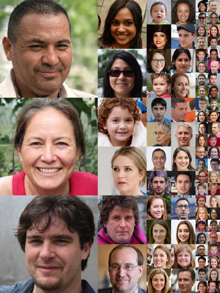
None of the human faces in figure 1 are real. They are all generated by a GAN. And they don’t look fake from any angle. So, this is the height of realism that we are able to achieve today with GANs. Not only this, but there are also many more applications as well. We will take a look into those in this post as well.

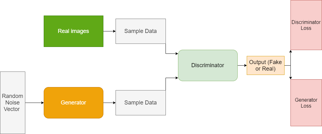
GANs Contain Two Neural Networks

GANs contail two neural network in their architecture. One is the generator and the other one is the discriminator.

While training a GAN, the generator tries to generate new fake data from a given noisy sample space. And with each iteration, it tries to generate more and more realistic data.

At the same time, the discriminator tries to differentiate the real data from the generated fake data of the generator. While training the discriminator, we provide it with both, the real data (positive examples) and the generated data (negative examples). A time will come when the discriminator won’t be able to tell whether the data is real or fake (generated by the generator). This is the time we stop the training and can successfully use the generator to generate realistic data that resembles the input data.

In the following two sections, we will be looking at the generator and discriminator in detail.

The Discriminator in GAN

The discriminator neural network in a GAN architecture tries to differentiate between the real data and the data generated by a generator. In fact, we can say that the discriminator is a binary classifier that classifies between positive and negative examples.

As such, the positive examples are the real data (with label 1) and the negative examples are the data generated by the generator (with label 0). If we take the example of image data, then the discriminator can be a convolutional neural network as well.

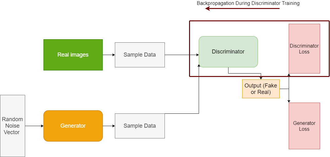
Figure 3 shows the flow of data and backpropagation when the discriminator is training.

Training the Discriminator

We already know that the discriminator uses two classes of data during its training. In the case of images, they are the real images and the fake images from the generator.

The important fact here is that while the discriminator trains, the generator does not train. While training the discriminator, we only backpropagate using the discriminator loss values. The loss values of the generator are frozen when the discriminator trains. We can also infer the same from figure 3.

Now, the real question is, how training the discriminator helps the generator?

Let’s take a look at that step by step.

• First, we give the real data and fake generator data as input to the discriminator.
• The discriminator classifies between fake data and real data. From this classification, we get the discriminator loss as we see in figure 3.
• If the discriminator misclassifies the data, then it is penalized. Misclassification can happen in two ways. Either when the discriminator classifies the real data as fake or when it classifies the fake data as real.
• In the final step, the weights get updated through backpropagation. Now, here is an important point to remember. The backpropagation in discriminator happens through the discriminator network. We will get to the importance of this point in the next section.

Apart from the above points, there is another important point to remember during the discriminator training. That is, the updated gradients from the discriminator training are not passed down to the generator.

Everything will become much clearer when get into the generator training part.

The Generator in GAN

The generator neural network tries to generate new data from the random noise (latent vector). With each iteration, it tries to produce more and more realistic data. These generated data also act as negative examples for the discriminator training. Also, the fake data generation process is linked to the feedback that the generator gets from the discriminator. As training progresses, the generator will eventually be able to fool the discriminator into classifying the fake data as real data.

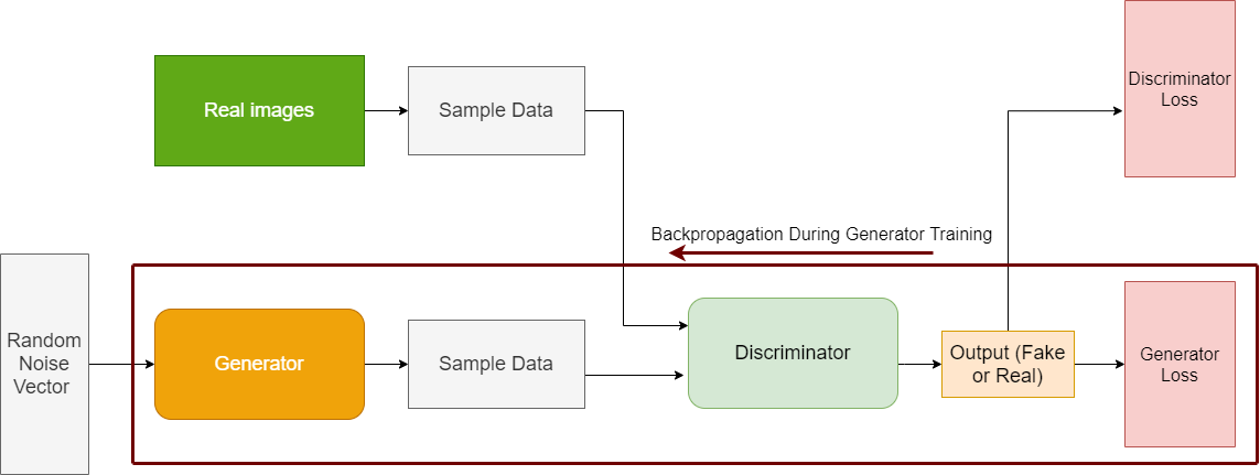
Figure 4 show the steps in GAN when the generator training happens.

Let’s get into details of generator training.

Training the Generator

The generator training goes through a number of steps. The following points will elaborate those:

• First, we have the random input or the latent vector or the noise vector.
• This random input is given to the generator and it generates the fake data.
• Then the discriminator network comes into play. At this step, the discriminator tries to classify the generated data as fake.
• We have the outputs from the discriminator which acts as a feedback to the generator. The discriminator feedback is used to penalize the generator for producing bad data instances.
• Also, we have the generator loss from the generator outputs. This generator loss penalizes the generator itself if it is not able to fool the discriminator.

Now, coming to some more important points. Take a look at figure 4 again. You can see that after we get the generator loss, the backpropagation happens both through the discriminator and the generator. We know that while training the generator and updating the weights we need to backpropagate through the generator. But why backpropagate through the discriminator also?

Although the discriminator parameters are frozen, still we need feedback about the performance of the generator. This we get by backpropagating through the discriminator also. The discriminator parameters do not get updated in this step but we get feedback about the generator.

This is one of the more important steps in GAN training. This is also the reason why GAN training is difficult. This means that it is difficult for a GAN to converge to an optimal solution. We will get into those details as well later in the article.

In the next section, we will take a look at the loss function(s) that is used in GANs.

Loss Function and Training of GANs

By now, we know that we need to train two neural networks to complete the GAN training. The generator and the discriminator train alternately. While the discriminator trains, the generator does not. Conversely, when the generator trains, the discriminator does not.

Also, training of GANs is a very difficult process and often not stable. There are many pitfalls and problems that we can face while trying to train GAN perfectly. We will get into those points. For now, we will focus on the loss function that is used to train GANs.

Loss Function in GANs

In this section, we will talk about the minimax loss that is described in the original paper on GANs.

First of all, let’s take a look at the loss function.

$$
\mathcal{L}(\theta^{(G)}, \theta^{(D)}) = \mathbb{E}_{x}logD(x) + \mathbb{E}_{z}(1 – D(G(z)))
$$

You may recognize the above loss function as a form of the very common binary-cross entropy loss. So, what do all the terms mean.

• \({E}_x\) is the expected value over all the data instances. You may recognize this as taking a sample from all the real images.
• \({E}_z\) is the expected value over the latent vector or the random noise vector that we give as input to the generator.
• \(D(x)\) corresponds to the probability by the discriminator that the given data \(x\) is real.
• \(G(z)\) is the data generated by the generator when we give it \(z\) as the input.
• \(D(G(z))\) is the probability by the discriminator that the data generated by the generator (\(G(z)\)) is real.

In GAN training, optimizing the above loss function is a two-sum game for the generator and the discriminator. It is called minimax because the discriminator tries to maximize the \(logD(x)\) term. While at the same time, the generator tries to minimize the \(log(1 − D(G(z)))\) term. Now, the question is, why such minimizing and maximizing would lead to the convergence while training a GAN?

Why the MiniMax Training Works?

To answer this, let’s go to basics of GAN again.

Remember that while the discriminator trains, the generator does not train. Also, \(D(x)\) corresponds to the probability by the discriminator that the given data \(x\) is real. So, when the discriminator trains, to minimize the whole loss, we need to correctly identify the real data. This is the same as classifying \(D(x)\) as 1.0. Then we know that \(D(G(z))\) is the probability by the discriminator that the data generated by the generator (\(G(z)\)) is real. Which means that we want to maximize this term while training the generator. But again, to minimize the whole loss function, we need to minimize the \(log(1 − D(G(z)))\) term.

I hope that this clears things up about the loss function. You should know that using the above loss function as it has its demerits and often a modified version is used. But these are the basics and also the same as discussed in the original GAN paper by Goodfellow et al.

In the next section, we are going to take look at the common pitfalls and problems that we face while training a GAN.

The Difficulty with Training GANs

By now, you must have realized that training a GAN is not as easy as training some other simple classification deep learning models. We need the minimax training with alternating of the discriminator and the generator. Even then there is no guarantee that a GAN will converge after a specific number of iterations.

The following subsections lay out some of the problems and difficulties when training GANs.

Failing of Generator in the Early Stages of Training

In the early stages of training, the generator is obviously not so good at generating new data instances. At this stage, it is very easy for the discriminator to classify the fake data and real data. According to the paper, here, \(log(1 − D(G(z)))\) saturates and the generator does not learn anything. To avoid this, instead of minimizing \(log(1 − D(G(z)))\), we try to maximize \(logD(G(z))\). This will provide better gradients in the early stages of training and will not lead to any saturation.

Mode Collapse

While training GAN, the training of both, the discriminator and generator must be synchronized. If we keep on training the generator without updating the discriminator, then the generator will learn to generate the same example over and over again which fools the discriminator easily. This mainly happens when the generator samples the same \(z\) from \(x\).

In such a scenario, the discriminator might never learn. This leads to the generator learning only a few specific types of data points without any diversity. This called mode collapse or the Helvetica Scenario.

Vanishing Gradients

Vanishing gradients, in general, can be a problem with any deep neural network training. And this happens in GANs too. To counter the vanishing gradients problem, we can use the modified loss function that we have discussed above in the “Failing of Generator in the Early Stages of Training” section.

We will not go into much of the theoretical details in this section. If you want to learn a bit more, then you may take a look at this.

Different Types of GANs and Their Applications

In this section, we will take a look at the different types of applications and the GANs that are used for those applications.

Generating New Images

This is perhaps one of the most common and popular usages of GANs. Using GANs, we can generate very high quality images from a given image dataset. But those images will be completely new and unseen.

GANs can nowadays generate very realistic but fake images of people who are hard to distinguish from real people.

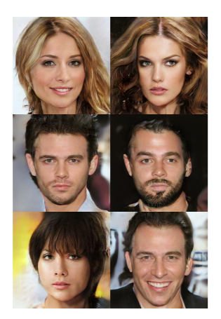
Figure 5 shows the image generation capability of GANs from the paper Progressive Growing of GANs for Improved Quality, Stability, and Variation.

This has become even better after the success of different GAN architectures like the progressive and conditional GANs.

Text-to-Image Synthesis

There are also variations of GANs that given a text input can produce images which resemble the text.

Let’ take a look at an example from the paper StackGAN: Text to Photo-realistic Image Synthesis with Stacked Generative Adversarial Networks.

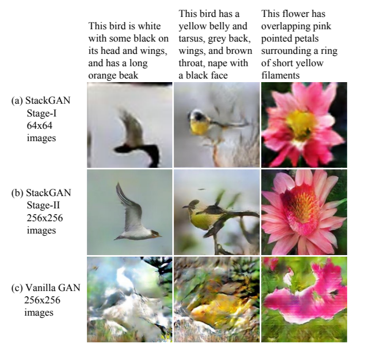
It is really impressive how accurate StackGAN is producing the images that match the texts. We can also see that it is far superior to other types of GANs like the Vanilla GAN.

Image Colorization and Image-to-Image Translation

We can also colorize sketches using GANs. The paper Image-to-Image Translation with Conditional Adversarial Networks is one of the best in this regard. Among many use cases, this paper also shows how we can give a sketch as input to a GAN and the GAN would colorize the sketch and produce a 3D image of the sketch as well.

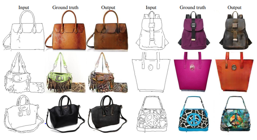
Figure 7 shows how the GAN can produce 3D outputs when given just sketches of handbags and bags.

Some other translation tasks also include:

• Weather translation in images.
• Day to night translation images.
• Aerial to map view translation.
• Segmentation to colored images translation.

You can find a full range of application in this paper.

Image Super-Resolution

Image super-resolution is another great use case of GANs. In image super-resolution, first, we give the GAN a very blurry low-resolution image as input. Then the GAN would produce a very crisp and high-resolution image as the output.

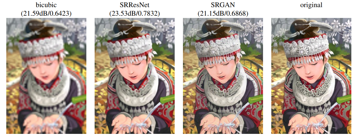
Figure 8 shows the results of image super-resolution using GAN from the paper Photo-Realistic Single Image Super-Resolution Using a Generative Adversarial Network. It is really amazing how effective the GAN architecture is at producing high-resolution images from low-resolution images.

There are many other application of GANs as well. Some of them include:

• Face in-painting.
• Text-to-speech.
• Generating realistic human faces.
• Video prediction.
• Cloth translation.
• Pose generation.

You can find details about the above in this amazing post by Jason Brownlee.

Links to Resources

• Book – Advanced Deep Learning with Keras – Chapter 4.
• Tutorial – Google Developers – GANs.
• Paper – Generative Adversarial Networks.
• Paper- UNROLLED GENERATIVE ADVERSARIAL NETWORKS.
• Paper – StackGAN: Text to Photo-realistic Image Synthesis with Stacked Generative Adversarial Networks.
• Paper – Image-to-Image Translation with Conditional Adversarial Networks.
• Paper – Photo-Realistic Single Image Super-Resolution Using a Generative Adversarial Network.

Summary and Conclusion

In this article, you learned about Generative Adversarial Networks in Deep Learning. In specific you learned about:

• The generator.
• The discriminator.
• Training of GANs and the loss function used.
• Problems in training GANs.
• And the use cases of GANs.

In the next tutorial, we will have hands-on experience and build our own GAN using PyTorch.

If you have any thoughts, doubts, or suggestions, then please use the comment section. I will surely address them.

You can contact me using the Contact section. You can also find me on LinkedIn, and Twitter.