Effective Model Saving and Resuming Training in PyTorch

In this tutorial, we will be taking a look at how to train and save deep learning neural network models effectively. Specifically, we will learn how to effectively do model saving and resuming training using PyTorch. We will also learn how to resume training after we load a trained model from disk using PyTorch.

In deep learning, after we collect and prepare the data that we have to use, it all comes down to one thing. Training our deep learning model and getting good training and validation results. Along with that, we also need good results when we give real-world data as input to the deep learning neural network model.

This tutorial has a two step structure. In the first step we will learn how to properly save the model in PyTorch along with the model weights, optimizer state, and the epoch information. The second step will cover the resuming of training. All in all, properly saving the model will have us in resuming the training at a later strage.

The Long Training Times of Deep Learning Models

Many times the above training and validation steps take a lot of time. For some deep learning research works, it can also mean training a neural network model for months. This is mostly the case when the researchers are trying to solve a novel task using deep learning that has not been solved before. So, don’t get astonished when you read in a paper that “the model was trained for 1.5 months on two Nvidia RTX 2080Ti”.

This all sounds great, but that does not mean we have to continuously train our deep learning model for 1.5 months to get good results. If you are an individual, then it is very unlikely that you are doing any such project that takes a neural network model 1.5 months to train.

But sometimes personal and individual projects involve a lot of training and validation procedures for deep learning models. That’s why knowing about proper model saving and resuming training is important.

Why the Longer Training and Validation Time?

There are mainly two reasons for such long training times:

• The dataset that we are using to train the deep learning model is huge. Maybe nearing 100s of gigabytes.
• The neural network model that is being trained is also huge. Maybe this contains a lot of layers.

The above two are the most common reasons for the long training times of deep learning models.

Why Longer Training Times for Deep Learning Models is a Problem?

Consider a few deep learning researchers trying to solve a problem using deep learning. Most of the time, they have a research grant for carrying out the research. And this grant almost always covers all the computational resources and expenses.

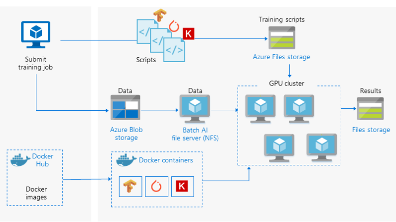
But as an individual, what can you do when you do not have such computational resources at hand. And I am pretty sure that you do not have a setup as shown in figure 2 at your disposal. Then how do you train your models for a long time?

There are a few steps that can help us to train our models for much longer than expected.

• First, we need an effective way to save the model. This includes saving the trained weights and the optimizer’s state as well.
• Then we need a way to load the model such that we can again continue training where we left off.

By using the above two steps, we can train our models longer and on more data as well. Now, I am not saying we need to train the model for months. But some individual projects may require a few days of training as well. So, the above techniques will help us a lot. And we will learn how to do those in this tutorial – all through hands-on and practical coding.

Model Saving and Resuming Training in PyTorch

Using state_dict to Save a Model in PyTorch

Basically, there are two ways to save a trained PyTorch model using the torch.save() function.

• Saving the entire model: We can save the entire model using torch.save(). The syntax looks something like the following.

# saving the model
torch.save(model, PATH)

# loading the model
model = torch.load(PATH)

But saving and loading the trained model like this does not leave us with much flexibility to refactor the code or use the trained model in some other projects. You can read more about it here.

• Saving the trained model parameters: Instead of saving the entire model, we can save the trained model parameters. For that, we need the save the model’s state_dict.

# save the model state_dict
torch.save(model.state_dict(), PATH)

# initialize the model class before loading the model
model = TheModelClass()
# load the model
model.load_state_dict(torch.load(PATH))

With this approach, first we need to initialize the model class before loading the model. Then we deserialize the model using torch.load(). After that, we load the learned parameters using model.load_state_dict().

The state_dict saving and loading are going to be the basis for loading our trained model and again resuming training.

Before that, a bit of setting up the project.

Setting Up the Project

We will use the CIFAR10 dataset in this tutorial. I know that the dataset is not large enough to show off the usefulness of model saving and resuming training. But after learning it here, you can apply the technique to any large project that you want.

And obviously, we will be using the PyTorch deep learning framework for this project.

Now, let’s take a look at the project structure.

├───input
├───outputs
└───src
│   initial_training.py
│   model.py
│   prepare_data.py
│   resume_training.py
│   utils.py

• The input folder will contain the CIFAR10 dataset that we will download using the datasets module of torchvision.
• The outptus folder will contain all the files that we will save during training and validation.
• We have five python scripts inside the src folder. They are initial_training.py, model.py, prepare_data.py, resume_training.py, and utils.py. We will go over the details of each of these scripts when we write the code for them.

For now, just prepare your directory like shown above and you are all set to follow along. We will start coding from the next section.

Preparing Our Deep Learning Neural Network Model

In this section, we will write the code to build the deep learning neural network model that we will use for training.

The code in this section will go into the model.py file inside the src folder. So, create the model.py file if you have not done so already. After writing the code here, we can import it to whichever other python scripts we want.

Importing the Modules

First, we need to import the modules and libraries that we need to build the neural network model.

import torch.nn as nn
import torch.nn.functional as F

We just need the above two for building the neural network model.

Next, we will create a Python class and call it CNN() which will be the name of our model.

The CNN() Neural Network Class

Here, we will write the whole neural network class code in one block of code. This will maintain the continuity of the code and make it easy to understand.

The neural network architecture is going to be very simple. This is because it is not our main focus here. Our aim is to learn how to save PyTorch models effectively and again load them to resume training. The following is the neural network model.

# model
class CNN(nn.Module):
    def __init__(self):
        super(CNN, self).__init__()
        self.conv1 = nn.Conv2d(in_channels=3, out_channels=64, kernel_size=5, padding=1)
        self.conv2 = nn.Conv2d(in_channels=64, out_channels=64, kernel_size=5, padding=1)
        self.conv3 = nn.Conv2d(in_channels=64, out_channels=128, kernel_size=5, padding=1)
        self.pool = nn.MaxPool2d(3, 2)
        self.dropout = nn.Dropout2d(0.5)
        self.fc1 = nn.Linear(in_features=128, out_features=1000)
        self.fc2 = nn.Linear(in_features=1000, out_features=10)

    def forward(self, x):
        x = F.relu(self.conv1(x))
        x = self.dropout(x)
        x = self.pool(x)
        x = F.relu(self.conv2(x))
        x = self.pool(x)
        x = F.relu(self.conv3(x))
        x = self.pool(x)
        # get the batch size and reshape
        bs, _, _, _ = x.shape
        x = F.adaptive_avg_pool2d(x, 1).reshape(bs, -1)
        x = F.relu(self.fc1(x))
        x = self.dropout(x)
        out = self.fc2(x)
        return out

• We have a total of three 2D convolutional layers and two fully connected layers.
• In the forward() function (starting from line 13):
  • We apply the ReLU activation to each layer (both convolutional and fully connected) except the last layer.
  • We also apply 2D Max-Pooling after each of the three convolutional layers.
  • There is also dropout regularization after the first convolutional layer (line 15) and the first fully connected layer (line 25).

The neural network model is very simple as we will be training the CIFAR10 dataset in this tutorial.

Prepare the Training and Validation Data

We will prepare a different python script for training and validation data. Doing so will allow us to import the data into other python scripts without repeating the code.

As you know, we will train our model twice in this tutorial. For that, we will need two different python script files. And while doing that, we do not want to repeat the data preparation code twice. Therefore, we are preparing the data in prepare_data.py which we can import anywhere we want.

So, the code from here on will go into the prepare_data.py file inside the src folder.

Let’s start with the imports.

from torchvision import datasets
from torchvision.transforms import transforms

We will download the CIFAR10 dataset using the datasets module from torchvision. Also, we will apply some data transformations to the images. Therefore, we import transforms as well.

Define the Training and Validation Transforms

We will define the image transforms for training data and validation data separately.

# define transforms
transform_train = transforms.Compose([
            transforms.RandomCrop(32, padding=4),
            transforms.RandomHorizontalFlip(),
            transforms.ToTensor(),
            transforms.Normalize((0.4914, 0.4822, 0.4465), 
                                 (0.2023, 0.1994, 0.2010)),
        ])

transform_val = transforms.Compose([
    transforms.ToTensor(),
    transforms.Normalize((0.4914, 0.4822, 0.4465), 
                         (0.2023, 0.1994, 0.2010)),
])

• For training data transforms (starting from line 2), first, we randomly crop the images. Then we flip the images horizontally randomly. Finally, we convert the pixels to tensors and normalize them.
• For the validation transforms (line 10), we just convert the images to tensors and normalize them.

CIFAR10 Training and Validation Data

Now, we will download the CIFAR10 dataset using the datasets module.

We will call the training data as train_data and validation data as val_data.

# train and validation data
train_data = datasets.CIFAR10(
    root='../input/data',
    train=True,
    download=True,
    transform=transform_train
)
val_data = datasets.CIFAR10(
    root='../input/data',
    train=False,
    download=True,
    transform=transform_val
)

The dataset will get downloaded into the input/data/ folder. Note that we apply the image transformations to the respective datasets.

This marks the end of our data preparation part.

Writing the Training and Validation Functions in utils.py

As you may have seen in the project structure section, we have utils.py file as well. We will write the training and validation function codes in this file. The reason is again the same. As we will train our model twice, we do not want to repeat the training and validation functions in the two files. We will write once in the utils.py file and import those.

The following block of code handles imports and defines the computation device.

from tqdm import tqdm

import torch

device = torch.device('cuda' if torch.cuda.is_available() else 'cpu')

It is better to have a GPU at your disposal for training deep neural networks. If you do not have one, you can always use Google Colab or Kaggle Kernels for training neural networks.

Define the Training Function

Here, we will define the training function. We will call it fit(). We will not go into much details about the function. It is very similar to other PyTorch training functions that you may have worked on before.

# training function
def fit(model, dataloader, optimizer, criterion, train_data):
    print('Training')
    model.train()
    train_running_loss = 0.0
    train_running_correct = 0
    for i, data in tqdm(enumerate(dataloader), total=int(len(train_data)/dataloader.batch_size)):
        data, target = data[0].to(device), data[1].to(device)
        optimizer.zero_grad()
        outputs = model(data)
        loss = criterion(outputs, target)
        train_running_loss += loss.item()
        _, preds = torch.max(outputs.data, 1)
        train_running_correct += (preds == target).sum().item()
        loss.backward()
        optimizer.step()
        
    train_loss = train_running_loss/len(dataloader.dataset)
    train_accuracy = 100. * train_running_correct/len(dataloader.dataset)    
    return train_loss, train_accuracy

The parameters for the fit() function are :

• The neural network model.
• The dataloader (training data loader).
• The optimizer.
• The criterion (loss function).
• The training data set.

We will pass these as arguments while calling the fit() function. The function returns the accuracy and loss after each epoch.

The Validation Function

We will call the validation function as validate(). This is going to be very similar to the training function.

# validation function
def validate(model, dataloader, optimizer, criterion, val_data):
    print('Validating')
    model.eval()
    val_running_loss = 0.0
    val_running_correct = 0
    with torch.no_grad():
        for i, data in tqdm(enumerate(dataloader), total=int(len(val_data)/dataloader.batch_size)):
            data, target = data[0].to(device), data[1].to(device)
            outputs = model(data)
            loss = criterion(outputs, target)
            
            val_running_loss += loss.item()
            _, preds = torch.max(outputs.data, 1)
            val_running_correct += (preds == target).sum().item()
        
        val_loss = val_running_loss/len(dataloader.dataset)
        val_accuracy = 100. * val_running_correct/len(dataloader.dataset)        
        return val_loss, val_accuracy

Just like the training function, validate() also returns the loss and accuracy after each epoch.

At this phase, we have completed all the preliminary coding requirements. Now, we can move on to training our neural network model.

Training our Neural Network Model for the First Time

To know how to resume training after loading a trained model, first, we need to save a model. For that, we need to train the neural network model. This is what we are going to do in this section of the tutorial.

We will train our CNN() neural network model on the training data only. We will not use the validation data. After training and saving the model, we will again load the model. Then we will train the model again and validate as well.

Let’s get started with the first phase of training. The code in this section will go into the initial_training.py file.

As always, we will start with the imports.

# imports
import torch
import torch.nn as nn
import torch.nn.functional as F
import numpy as np
import matplotlib.pyplot as plt
import matplotlib
import torch.optim as optim
import model

from torch.utils.data import DataLoader
from prepare_data import train_data
from utils import fit

matplotlib.style.use('ggplot')

• At line 12, we import the train_data only from prepare_data. This is because we will only be training, not validating.
• Similarly, we import the fit function only from utils.

Define the Learning Parameters and the Train Loader

Here, we will define the learning parameters and the train data loader.

# learning parameters
batch_size = 128
epochs = 10
lr = 0.001
device = torch.device('cuda' if torch.cuda.is_available() else 'cpu')

# train data loader
train_loader = DataLoader(
    train_data, 
    batch_size=batch_size,
    shuffle=True
)

• We will be using a batch size of 128. As the images are only 32×32 pixels in size, we can easily use a batch size of 128.
• The number of epochs is 10.
• The learning rate is 0.001.
• At line 8, we define the train_loader. We are shuffling the train_loader also.

Initialize the Model Class, the Optimizer, and the Loss Function

The model file is already imported at the beginning of the script. We just need to initialize it here and load it onto the computation device.

# initialize the model
model = model.CNN().to(device)
# optimizer and loss function
optimizer = optim.Adam(model.parameters(), lr=lr, betas=(0.9, 0.999), 
                       eps=1e-8, weight_decay=0.0005)
criterion = nn.CrossEntropyLoss()

• The model initialization happens on line 2.
• We are using the Adam optimizer that we initialize at line 4.
• Line 5 defines the CrossEntropyLoss for training our deep neural network model.

We can also print the check the model’s and optimizer’s initial state_dict. And by initial, we mean before we carry out the training. The following block of code shows how to print the state_dict of the model and the optimizer.

# model's state_dict
for param_tensor in model.state_dict():
    print(f"{param_tensor} \t {model.state_dict()[param_tensor].size()}")
# optimizer's state_dict
for var_name in optimizer.state_dict():
    print(f"{var_name} \t {optimizer.state_dict()[var_name]}")

We just need to use the model.state_dict() and optimizer.state_dict() and print the values at the param_tensor index. We have done so at lines 3 and 6.

Execute the fit() Function

While importing the modules, we have also imported the fit() function from utils. To carry out training, we just need to call the fit() function for 10 epochs.

train_loss , train_accuracy = [], []
for epoch in range(epochs):
    print(f"Epoch {epoch+1} of {epochs}")
    train_epoch_loss, train_epoch_accuracy = fit(model, train_loader, 
                                                 optimizer, criterion, 
                                                 train_data)
    train_loss.append(train_epoch_loss)
    train_accuracy.append(train_epoch_accuracy)
    print(f"Train Loss: {train_epoch_loss:.4f}, Train Acc: {train_epoch_accuracy:.2f}")

In the above block, at line 1, we have the train_loss and train_accuracy lists. We append the epoch-wise loss and accuracy values to both these lists respectively (lines 7 and 8).

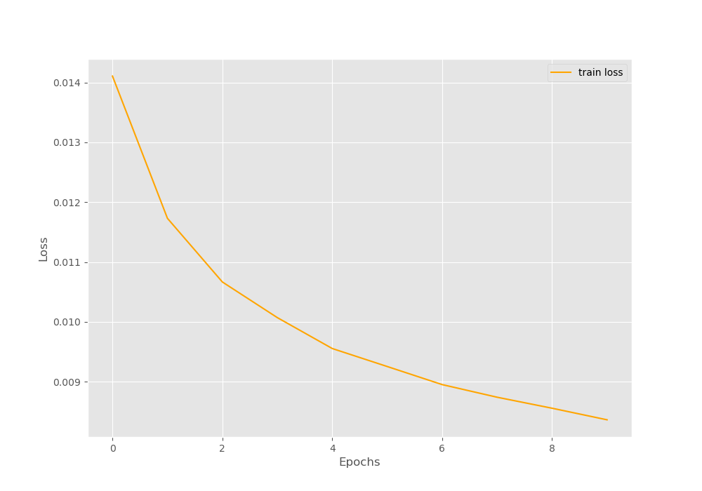
Further on, we should also save the line plots of the accuracy and loss values for the 10 epochs. This will help us in analyzing the results later.

# accuracy plots
plt.figure(figsize=(10, 7))
plt.plot(train_accuracy, color='green', label='train accuracy')
plt.xlabel('Epochs')
plt.ylabel('Accuracy')
plt.legend()
plt.savefig('../outputs/initial_training_accuracy.png')
plt.show()
 
# loss plots
plt.figure(figsize=(10, 7))
plt.plot(train_loss, color='orange', label='train loss')
plt.xlabel('Epochs')
plt.ylabel('Loss')
plt.legend()
plt.savefig('../outputs/initial_training_loss.png')
plt.show()

The accuracy plot will be saved as initial_training_accuracy.png in the outputs folder. And the loss plot will be saved as initial_training_loss.png.

Saving the Model Checkpoint

As we have to resume training later, we also have to save the checkpoint of our trained deep neural network. We can resume training only of we have a saved checkpoint with all the trained parameters. We need to load the trained parameters and then resume training again.

The following block of code shows how to do it.

# save model checkpoint
torch.save({
            'epoch': epochs,
            'model_state_dict': model.state_dict(),
            'optimizer_state_dict': optimizer.state_dict(),
            'loss': criterion,
            }, '../outputs/model.pth')

Let’s go over the code in the above block.

• We use the torch.save() function as usual. But instead of saving just the model’s state_dict, we also save a bunch of other information. And we do that in dictionary form.
• The first key-value pair is the number of epochs ('epoch') that we trained the model for. Although this is not directly necessary for resuming training, still we will have the information of the previous training epochs.
• The second key is 'model_state_dict' and its value is model_state_dict(). This saves the trained neural network parameters.
• Next is the 'optimizer_state_dict'. We also save this with the values as optimizer.state_dict(). For resuming training, we also need the optimizer’s state_dict.
• And the last one is the loss. We need to know what loss function was used before we resume training.
• Finally, we give the path where the model is saved. The models is saved as model.pth in the outputs folder.

We have completed writing the code for the first phase of training our deep neural network. After proper model saving, next comes the resuming of training by loading the already trained model.

Writing the Code to Resume Training in PyTorch

After saving the model properly, let’s learn how resuming training helps to train neural networks longer. The code in this section will go into the resume_training.py file inside the src folder. This time, we will carry out both, training and validation. So, we will use the training data and the validation data as well.

I hope that you have created the python file before moving further.

First, of all we need to import all the modules and libraries.

# imports
import torch
import torch.nn as nn
import torch.nn.functional as F
import numpy as np
import matplotlib.pyplot as plt
import matplotlib
import torch.optim as optim
import model

from torch.utils.data import DataLoader
from tqdm import tqdm
from prepare_data import train_data, val_data
from utils import fit, validate

matplotlib.style.use('ggplot')

• Note that at line 13, we are importing the train_data and val_data. Also, at line 14, we are importing fit and validate from utils. This is because along with resuming training, we will validate our neural network model as well.

Next, we will define some of the learning parameters as we did in the case of the initial training phase.

# learning parameters
batch_size = 128
new_epochs = 10
lr = 0.001
device = torch.device('cuda' if torch.cuda.is_available() else 'cpu')

At line 3, we define new_epochs. We will again train the model for 10 epochs while executing this python script.

Initializing the Model Class and Loading the Saved state_dict

This is the most important part of code when we want to resume training. First, we will initialize the neural network model class to load the model architecture. Along with that, we will also initialize the optimizer. We will again initialize the Adam optimizer.

# load the trained model
model = model.CNN().to(device) # initilize the model
# initialize optimizer  before loading optimizer state_dict
optimizer = optim.Adam(model.parameters(), lr=lr, 
                       betas=(0.9, 0.999), 
                       eps=1e-8, weight_decay=0.0005)

The next few lines of code are really important. We load the model checkpoint and along with that all the previously saved state_dict as well.

# load the model checkpoint
checkpoint = torch.load('../outputs/model.pth')
# load model weights state_dict
model.load_state_dict(checkpoint['model_state_dict'])
print('Previously trained model weights state_dict loaded...')
# load trained optimizer state_dict
optimizer.load_state_dict(checkpoint['optimizer_state_dict'])
print('Previously trained optimizer state_dict loaded...')
epochs = checkpoint['epoch']
# load the criterion
criterion = checkpoint['loss']
print('Trained model loss function loaded...')

print(f"Previously trained for {epochs} number of epochs...")
# train for more epochs
epochs = new_epochs
print(f"Train for {epochs} more epochs...")

• At line 2, first, we load the model checkpoint from the previously trained model.
• Then at line 4, we load the state_dict from the checkpoint to the initialized model, that is model.
• Line 7 loads the saved optimizer’s state_dict on to the newly initialized optimizer.
• Then at line 9, we get the number of epochs that the model was previously trained for.
• Line 11 loads the loss function from the checkpoint as criterion .
• Finally, line 16, assigns the new number of epochs to the epochs variable. So, we will again train our model for 10 epochs.

In the above code block, we print some information after each step so that we know exactly what is happening.

Prepare the Train and Validate Data Loaders

We will prepare the train and validation data loaders. The validation data loader is the extra here.

# train data loader
train_loader = DataLoader(
    train_data, 
    batch_size=batch_size,
    shuffle=True
)
val_loader = DataLoader(
    val_data,
    batch_size=batch_size,
    shuffle=False
)

We are not shuffling the val_loader.

Training and Validation for 10 Epochs

Along with the fit() function, we will also call the validate() function this time. So, we will carry out both, training and validation for 10 epochs.

train_loss , train_accuracy = [], []
val_loss , val_accuracy = [], []
for epoch in range(epochs):
    print(f"Epoch {epoch+1} of {epochs}")
    train_epoch_loss, train_epoch_accuracy = fit(model, train_loader, 
                                                 optimizer, criterion, 
                                                 train_data)
    val_epoch_loss, val_epoch_accuracy = validate(model, val_loader, 
                                                 optimizer, criterion, 
                                                 val_data)
    train_loss.append(train_epoch_loss)
    train_accuracy.append(train_epoch_accuracy)
    val_loss.append(val_epoch_loss)
    val_accuracy.append(val_epoch_accuracy)
    print(f"Train Loss: {train_epoch_loss:.4f}, Train Acc: {train_epoch_accuracy:.2f}")
    print(f'Val Loss: {val_epoch_loss:.4f}, Val Acc: {val_epoch_accuracy:.2f}')

We are using val_loss and val_accuracy lists to append the validation loss and accuracy values after each epoch.

Saving the Line Plots and Model Checkpoint

The next block of code saves the line plots for the loss and accuracy values for validation and training.

# accuracy plots
plt.figure(figsize=(10, 7))
plt.plot(train_accuracy, color='green', label='train accuracy')
plt.plot(val_accuracy, color='blue', label='validataion accuracy')
plt.xlabel('Epochs')
plt.ylabel('Accuracy')
plt.legend()
plt.savefig('../outputs/resume_training_accuracy.png')
plt.show()
 
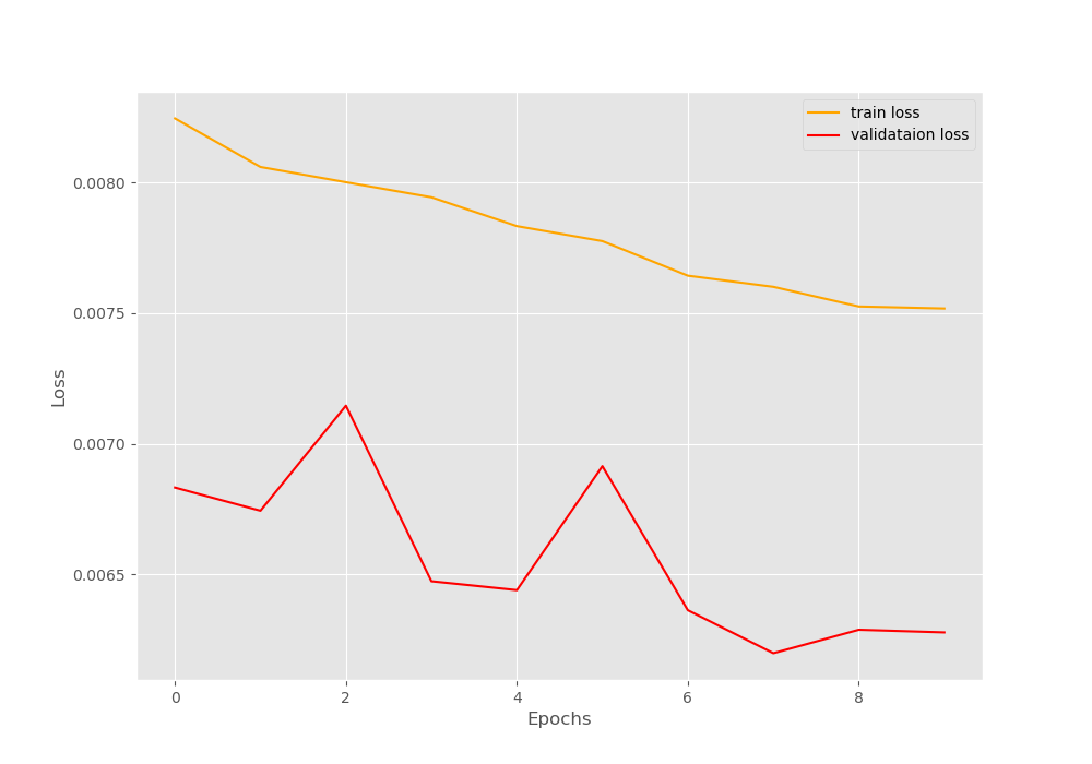
# loss plots
plt.figure(figsize=(10, 7))
plt.plot(train_loss, color='orange', label='train loss')
plt.plot(val_loss, color='red', label='validataion loss')
plt.xlabel('Epochs')
plt.ylabel('Loss')
plt.legend()
plt.savefig('../outputs/resume_training_loss.png')
plt.show()

Finally, we will again save the model checkpoint along with all the information, just like last time.

# save model checkpoint
torch.save({
            'epoch': epochs,
            'model_state_dict': model.state_dict(),
            'optimizer_state_dict': optimizer.state_dict(),
            'loss': criterion,
            }, '../outputs/model.pth')

This marks the end of all the code that we need to write.

We now just need to execute both the python training scripts and see how everything works out.

Execute the initial_training.py File

To execute the python training scripts you need to be in the src folder in the terminal. Now, type the following command.

python initial_training.py

You should see an output similar to the following.

conv1.weight     torch.Size([64, 3, 5, 5])
conv1.bias       torch.Size([64])
conv2.weight     torch.Size([64, 64, 5, 5])
conv2.bias       torch.Size([64])
conv3.weight     torch.Size([128, 64, 5, 5])
conv3.bias       torch.Size([128])
fc1.weight       torch.Size([1000, 128])
fc1.bias         torch.Size([1000])
fc2.weight       torch.Size([10, 1000])
fc2.bias         torch.Size([10])
state    {}
param_groups     [{'lr': 0.001, 'betas': (0.9, 0.999), 'eps': 1e-08, 'weight_decay': 0.0005, 'amsgrad': False, 'params': [1286724060808, 1286724060888, 1286724061048, 1286724061128, 1286724061288, 1286724061368, 1286724061448, 1286724061528, 1286724061608, 1286724061688]}]
Epoch 1 of 10
Training
391it [00:23, 16.29it/s]
Train Loss: 0.0141, Train Acc: 33.56
...
Epoch 10 of 10
Training
391it [00:16, 23.16it/s]
Train Loss: 0.0084, Train Acc: 62.93

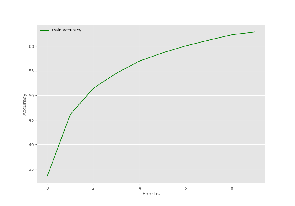
First, the output shows the state_dict of the model and the optimizer. Then we have the epoch-wise accuracy values. After the first epoch, the accuracy is 33.56%. And we have an accuracy of 62.93% after the 10\(^{th}\) epoch. Our aim here is not to get a very high accuracy. We need the accuracy values to know whether we are actually able to resume training the model or not.

For just a bit more clarity, let’s visualize the accuracy line plot as well.

Now, let’s execute the resume_training.py file.

Execute the resume_training.py File

Let’s hope that after executing the resume_training.py file, the training will continue where we left off. Remember that this time both training and validation will take place for 10 epochs.

python resume_training.py

The following is the truncated output while executing the file.

Previously trained model weights state_dict loaded...
Previously trained optimizer state_dict loaded...
Trained model loss function loaded...
Previously trained for 10 number of epochs...
Train for 10 more epochs...
Epoch 1 of 10
Training
391it [00:17, 22.53it/s]
Validating
79it [00:02, 32.29it/s]
Train Loss: 0.0082, Train Acc: 63.78
Val Loss: 0.0068, Val Acc: 71.09
...
Epoch 10 of 10
Training
391it [00:17, 22.49it/s]
Validating
79it [00:02, 34.93it/s]
Train Loss: 0.0075, Train Acc: 66.82
Val Loss: 0.0063, Val Acc: 73.01

The training starts after printing all the information on the terminal. You can see that the accuracy after the first epoch is 63.78%. Remember that after the initial training’s last epoch the accuracy was 62.93%. This shows that the training actually resumed after loading all the state_dict properly. Although the validation accuracy is higher than the training accuracy, it is not much of a concern here. This is most probably due to the lack of data augmentation. After the last epoch, the training accuracy is 66.82% and the validation accuracy is 73.01%.

Let’s visualize the line plots for a bit more clarity.

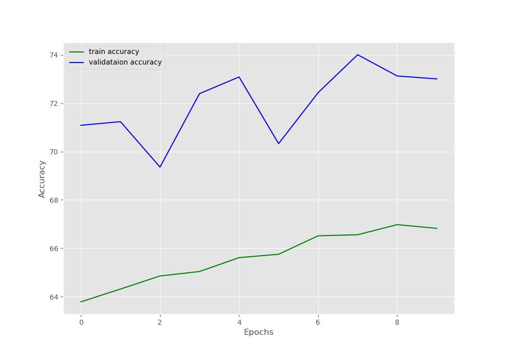
The line plots also show the same thing about the training and validation accuracy values.

This shows that we can very easily resume training if we have limited compute for deep learning training. We can train our deep neural network model for some epochs and then resume training at a later stage. This will allow to train the neural network in multiple phases without worrying much about longer training times.

Summary and Conclusion

In this tutorial, you learned how longer training times of deep neural networks can be a problem for large-scale projects. We need much more computing power for that. Then you learned how we can tackle the problem by saving the model checkpoint and then again resuming training at a later stage. I hope that this tutorial helped you to expand your knowledge about deep learning and neural network training.

If you have any doubts, thoughts, or suggestions, then leave them in the comment section. I will surely address them.

You can contact me using the Contact section. You can also find me on LinkedIn, and Twitter.