Face Image Generation using Convolutional Variational Autoencoder and PyTorch

In this tutorial, you will learn about convolutional variational autoencoder. Specifically, you will learn how to generate new images using convolutional variational autoencoders. We will be using the Frey Face dataset in this tutorial.

In the previous article, I showed how to get started with variational autoencoders in PyTorch. The article covered the basic theory and mathematics behind the implementation of the variational autoencoder. If you read that article, then you will also learn how to generate new digits by training a simple linear VAE on the MNIST digit dataset.

If you are new to autoencoders in general, then I recommend that you through the autoencoders section first, then come back to this article. By going through some of the previous articles on autoencoders, you will learn the following.

• Basic theory on autoencoders.
• Implementing simple linear and convolutional autoencoders on both, greyscale and color images.
• Using autoencoders to denoise images.
• Implementing variational autoencoders using the PyTorch deep learning framework.

What will you learn in this tutorial?

• Getting to know about the Frey Face dataset.
• Getting started with convolutional variational neural network on greyscale images.
• Using the VAE network to train on the Frey Face dataset and generating new face images.

Now, let’s put all our focus on this tutorial and get to know a bit more about the dataset that we will be using.

The Frey Face Dataset

You will find the Frey Face dataset on this page. The Frey Face dataset is a very common dataset that is used in the deep learning community to test generative neural network models like VAEs, and GANs (Generative Adversarial Networks).

The following is the definition of the dataset according to the webpage.

From Brendan Frey. Almost 2000 images of Brendan’s face, taken from sequential frames of a small video. Size: 20×28.

So, the dataset contains around 2000 face images. The images are 28 pixels in height and 20 pixels in width. All of the images are in grayscale format. This means that the number of color channels in 1.

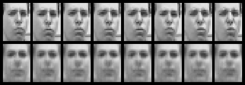
Now, let’s take a look at some of the images in the dataset. This will give us a better idea of the images that we will be using.

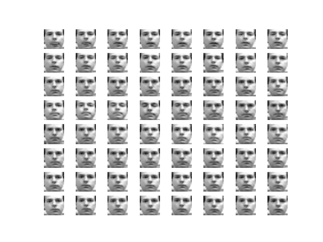
Figure 1 shows the face images in an 8×8 grid. There are some variations in each image, although not much.

One important question is, why this dataset for learning about convolutional autoencoders? There are some important reasons.

• First of all, the dataset is not that huge. Only around 2000 images which is good to start out with the concept.
• The images are in grayscale format having only one color channel. Also, the images are pretty simple. All the images are of faces with very slight variations from one another. This means that we do not need a very powerful neural network to learn the features of the images. This also means less fine-tuning and less training as well. This is just perfect for learning about convolutional variational autoencoders.

Download the Dataset

You can go ahead and download the dataset from here. The dataset that you are looking for is in the Faces section and named as Frey Face. A file with name frey_rawface.mat will download. It is a very small file, only around 1 MB.

The Deep Learning Framework and Project Structure

In this tutorial, we will use the PyTorch deep learning framework. If you do not have it already, then you can install PyTorch from here. If you are doing a fresh install, then I recommend that you create a new environment for this version of PyTorch. This will ensure that it does not conflict with other deep learning framework and projects that you have on your system.

Now, coming to the project structure. It is going to be very simple. The following is the project structure that we will be using{py}{/py}.

├───input
│       frey_rawface.mat
│
├───outputs
│
└───src
    │   model.py
    │   train.py

• In the input folder, we have the Frey Face dataset, that is, the frey_rawface.mat file.
• The outputs folder will contain the outputs that the code will generate while training the convolutional VAE model. This includes all the images that will be reconstructed by the VAE neural network model.
• src folder contains two python scripts. The model.py script will contain the convolutional VAE class code. And the train.py script will contain the python code to train the convolutional VAE neural network model on the Frey Face dataset.

I hope that you have set up the project structure like the above. We are all set to write the code and implement a convolutional variational autoencoder on the Frey Face dataset.

Implementing Convolutional Variational Autoencoder using PyTorch

From this section onward, we will focus on the coding and implementation part of the tutorial. We have two python scripts, one is model.py and the other is train.py. I will be indicating what code goes into which of the python scripts.

We will start with writing the code to create our convolutional variational autoencoder neural network.

Creating the Convolutional Variational Autoencoder Neural Network Model

We will create a very simple convolutional VAE model. The code in this section will go into the model.py file.

Note: We will not go into the detail working of the reparameterization trick, latent space mean, and log variance of the neural network. It is better if you read about those in the previous post. This is because I have explained those concepts in detail in that post. These concepts form the basis of the working of VAEs. So, it is better if you read about those concepts before moving further. However, I will be providing an ample explanation of the model that we will be creating.

So, open up the model.py file inside the src folder and follow along.

Imports for the model.py File

Let’s start with importing all the modules that we will need for creating our convolutional VAE neural network.

import torch
import torch.nn as nn
import torch.nn.functional as F

The above are all the imports that we need.

Next, let’s define the kernel size, the stride for convolutional blocks, padding, and the number of filters to start with.

kernel_size = 4
stride = 1
padding = 0
init_kernel = 16 # initial number of filters

• Each of the convolutional blocks will have a kernel size of 4×4 with stride 1 and no zero padding. Defining these here will make our work of building the convolutional VAE much easier for us. You will see shortly how to use these effectively. Also, the starting number of filters for the neural network will be 16, the init_kernel variable.

Define the Convolutional VAE Class in the model.py File

Here, we will define the convolutional VAE class that builds the model for us. We will call it as ConvVAE().

First, we will write the whole code defining the model, then we will move on to the explanation part. This will ensure that we have continuity in our code.

# define a Conv VAE
class ConvVAE(nn.Module):
    def __init__(self):
        super(ConvVAE, self).__init__()
 
        # encoder
        self.enc1 = nn.Conv2d(
            in_channels=1, out_channels=init_kernel, kernel_size=kernel_size, 
            stride=stride, padding=padding
        )
        self.enc2 = nn.Conv2d(
            in_channels=init_kernel, out_channels=init_kernel*2, kernel_size=kernel_size, 
            stride=stride, padding=padding
        )
        self.enc3 = nn.Conv2d(
            in_channels=init_kernel*2, out_channels=init_kernel*4, kernel_size=kernel_size, 
            stride=stride, padding=padding
        )
        self.enc4 = nn.Conv2d(
            in_channels=init_kernel*4, out_channels=init_kernel*8, kernel_size=kernel_size, 
            stride=stride, padding=padding
        )
        self.enc5 = nn.Conv2d(
            in_channels=init_kernel*8, out_channels=init_kernel, kernel_size=kernel_size, 
            stride=stride, padding=padding
        )

        # decoder 
        self.dec1 = nn.ConvTranspose2d(
            in_channels=init_kernel, out_channels=init_kernel*8, kernel_size=kernel_size, 
            stride=stride, padding=padding
        )
        self.dec2 = nn.ConvTranspose2d(
            in_channels=init_kernel*8, out_channels=init_kernel*4, kernel_size=kernel_size, 
            stride=stride, padding=padding
        )
        self.dec3 = nn.ConvTranspose2d(
            in_channels=init_kernel*4, out_channels=init_kernel*2, kernel_size=kernel_size, 
            stride=stride, padding=padding
        )
        self.dec4 = nn.ConvTranspose2d(
            in_channels=init_kernel*2, out_channels=init_kernel, kernel_size=kernel_size, 
            stride=stride, padding=padding
        )
        self.dec5 = nn.ConvTranspose2d(
            in_channels=init_kernel, out_channels=1, kernel_size=kernel_size, 
            stride=stride, padding=padding
        )

    def reparameterize(self, mu, log_var):
        """
        :param mu: mean from the encoder's latent space
        :param log_var: log variance from the encoder's latent space
        """
        std = torch.exp(0.5*log_var) # standard deviation
        eps = torch.randn_like(std) # `randn_like` as we need the same size
        sample = mu + (eps * std) # sampling
        return sample
 
    def forward(self, x):
        # encoding
        x = F.relu(self.enc1(x))
        x = F.relu(self.enc2(x))
        x = F.relu(self.enc3(x))
        x = F.relu(self.enc4(x))
        x = self.enc5(x)

        # get `mu` and `log_var`
        mu = x
        log_var = x

        # get the latent vector through reparameterization
        z = self.reparameterize(mu, log_var)
 
        # decoding
        x = F.relu(self.dec1(z))
        x = F.relu(self.dec2(x))
        x = F.relu(self.dec3(x))
        x = F.relu(self.dec4(x))
        reconstruction = torch.sigmoid(self.dec5(x))
        return reconstruction, mu, log_var

Explanation of the ConvVAE() Class

In the ConvVAE() class, starting from line 3, we have the __init__() function. In the __init__() function, we define all the encoder and decoder layers of our convolutional VAE neural network.

• Starting from line 7, we have the encoder layers. The input channels for the first encoder layer is 1 as all the images are greyscale images. As it is a convolutional VAE, all the encoder layers are 2D convolution layers.
• The output channels of self.enc1 is 16 that we defined above.
• After that, we double the number of output channels in each of the encoder layer till self.enc4. Here, we have 128 output channels.
• In the last encoder layer, that is line 23, we again have 16 output channels.
• All the encoder layers have a kernel size of 4×4 with stride 1. We are not providing zero padding for any of the layers. That is, padding=0 for all the layers.

Then starting from line 29, we define the decoder layers of the VAE neural network.

• For decoding, we use 2D transpose convolutions (ConvTranspose2d()).
• All the in_channels and out_channels are in reverse order with regard to the encoder layers.
• Again, all the decoder layers have 4×4 kernel size, stride as 1, and no zero padding.

From line 50, we have the reparameterize() function. This function returns the sample after calculating the standard deviation and epsilon values.

We have the forward() function starting from line 60.

• From lines 62 to 66, we get the encodings of all the image inputs by passing them through the encoder layers.
• Next, we get the mu and log_var from the encodings (lines 69 and 70). mu is the mean from the encoder’s latent space. And log_var is the log variance from the encoder’s latent space.
• Line 73 gives the latent vector z.
• Then from line 76, we have the decoder layers. The input to the first decoder layer at line 76 is the latent vector z.
• At line 80, we get the reconstruction from the last decoder layer. Finally, at line 81, we return the reconstruction, mu, and log_var.

Again, if you find any of the above confusing, then I highly recommend referring my previous post of variational autoencoders where I explain these in detail.

Writing the Code to Train the Convolutional Variational Autoencoder Neural Network on the Frey Face Dataset

Beginning from this section, we will write the code to train our ConvVAE() neural network on the Frey Face dataset. We will write the code in the train.py file. So, open up the train.py file inside the src folder and follow along.

Importing Modules and Defining the Training Parameters for the Convolutional VAE Neural Network

The following code block imports all the modules that we need for training our Convolutional VAE neural network.

import scipy.io
import torch
import torch.optim as optim
import torch.nn as nn
import model

from torch.utils.data import DataLoader, Dataset
from tqdm import tqdm
from torchvision.utils import save_image

At line 1, we import scipy.io. Remember that our data has a .mat extension. To read that file we need the scipy.io module.

For the learning parameters, we will define the batch size, the learning rate, number of epochs, and computation device.

# learning parameters
batch_size = 64
lr = 0.001
epochs = 20
device = torch.device('cuda' if torch.cuda.is_available() else 'cpu')

• We are using a batch size of 64. You can easily use a bigger batch size as the images are very small (20×28 pixels).
• The learning rate is 0.001.
• And we will be training the Convolutional VAE neural network for 20 epochs.
• For the computation device, it won’t matter much whether using a GPU or CPU for this dataset. This is because the dataset is very small and the images are very small as well. The training will finish within minutes even on the CPU.

Preparing the Frey Face Dataset

By default, the Frey Face dataset is a MAT-file dictionary. We can load it using the scipy.io module. The ff key contains the data values in the dictionary. For convenience, we will convert all the pixel values into NumPy array format.

# get the data into NumPy format
mat_data = scipy.io.loadmat('../input/frey_rawface.mat')
data = mat_data['ff'].T.reshape(-1, 1, 28, 20)
data = data.astype('float32') / 255.0
print(f"Number of instances: {len(data)}")

At line 3, we get the pixel values from the ff key and reshape the data into proper format. Line 4 divides all the values by 255.0 so that the pixels values are within 0.0 and 1.0 range.

We will divide the data into a training and a validation set. We will use 300 images for validation and the rest for training.

# divide the data into train and validation set
x_train = data[:-300]
x_val = data[-300:]
print(f"Training instances: {len(x_train)}")
print(f"Validation instances: {len(x_val)}")

Next, we will prepare our custom dataset module using the Dataset class from PyTorch. There is nothing fancy here. We will just be returning the images according to the indices. We do not have any labels in the dataset. So, that makes our work even easier. Let’s call the custom class as FreyDataset().

# prepare the torch Dataset
class FreyDataset(Dataset):
    def __init__(self, X):
        self.X = X

    def __len__(self):
        return (len(self.X))

    def __getitem__(self, index):
        data = self.X[index]
        return torch.tensor(data, dtype=torch.float)

Now, we will initialize the FreyDataset() with train_data and val_data. Finally, we will prepare the training and validation data loaders.

train_data = FreyDataset(x_train)
val_data = FreyDataset(x_val)

# iterable data loader
train_loader = DataLoader(train_data, batch_size=batch_size)
val_loader = DataLoader(val_data, batch_size=batch_size)

Initialize the Convolution VAE Neural Network Model

We have already imported the model at the beginning of the train.py script. Now, we just need to initialize the model and load it onto the computation device. Along with that, we will also define the optimizer and the reconstruction loss function.

model = model.ConvVAE().to(device)
optimizer = optim.Adam(model.parameters(), lr=lr)
criterion = nn.BCELoss(reduction='sum')

Note that the loss function (BCELoss) in the above code block is the reconstruction loss. This means that it will calculate the loss between the input image and the image reconstructed by the decoder. We will need to define the KL-Divergence loss as well. We will do that next.

Define the Final Loss Function

As discussed above, we will also need to define the KL-Divergence loss along with the reconstruction loss. The final loss will be the addition of the reconstruction loss and the KL-Divergence loss.

def final_loss(bce_loss, mu, logvar):
    """
    This function will add the reconstruction loss (BCELoss) and the 
    KL-Divergence.
    KL-Divergence = 0.5 * sum(1 + log(sigma^2) - mu^2 - sigma^2)

    :param bce_loss: recontruction loss
    :param mu: the mean from the latent vector
    :param logvar: log variance from the latent vector
    """
    BCE = bce_loss 
    KLD = -0.5 * torch.sum(1 + logvar - mu.pow(2) - logvar.exp())

    return BCE + KLD

I have provided documentation in the above code block for understanding as well.

If you need to know why we need the KL-Divergence as well, then do take a look at the previous post.

Define the Training Function

We will define the training function here. We will call it as fit(). It is a very simple training function and similar to most of the PyTorch training functions that you may have seen before.

def fit(model, dataloader):
    model.train()
    running_loss = 0.0
    for i, data in tqdm(enumerate(dataloader), total=int(len(train_data)/dataloader.batch_size)):
        data= data
        data = data.to(device)
        data = data
        optimizer.zero_grad()
        reconstruction, mu, logvar = model(data)
        bce_loss = criterion(reconstruction, data)
        loss = final_loss(bce_loss, mu, logvar)
        loss.backward()
        running_loss += loss.item()
        optimizer.step()

    train_loss = running_loss/len(dataloader.dataset)
    return train_loss

The only difference is that we calculate the total loss at line 11 by calling the final_loss() function. Line 17 returns the epoch-wise loss for each training epoch.

The Validation Function

The validation function will be very similar to the training function. But we need not backpropagate the gradients or update the parameters.

def validate(model, dataloader):
    model.eval()
    running_loss = 0.0
    with torch.no_grad():
        for i, data in tqdm(enumerate(dataloader), total=int(len(val_data)/dataloader.batch_size)):
            data= data
            data = data.to(device)
            data = data
            reconstruction, mu, logvar = model(data)
            bce_loss = criterion(reconstruction, data)
            loss = final_loss(bce_loss, mu, logvar)
            running_loss += loss.item()
        
            # save the last batch input and output of every epoch
            if i == int(len(val_data)/dataloader.batch_size) - 1:
                num_rows = 8
                both = torch.cat((data[:8], 
                                  reconstruction[:8]))
                save_image(both.cpu(), f"../outputs/output{epoch}.png", nrow=num_rows)

    val_loss = running_loss/len(dataloader.dataset)
    return val_loss

At line 15, we check whether we are at the last batch of the training epoch. If so, then we save the original image data and the reconstructed image. We use the save_image() function from torchvision. This allows us to easily save batch of images and concatenate the original image and reconstructed image as top and bottom rows.

Execute the fit() and validate() Functions

For the final part, we need to call the fit() and validate() functions. We will train and validate for 20 epochs.

train_loss = []
val_loss = []
for epoch in range(epochs):
    print(f"Epoch {epoch+1} of {epochs}")
    train_epoch_loss = fit(model, train_loader)
    val_epoch_loss = validate(model, val_loader)
    train_loss.append(train_epoch_loss)
    val_loss.append(val_epoch_loss)
    print(f"Train Loss: {train_epoch_loss:.4f}")
    print(f"Val Loss: {val_epoch_loss:.4f}")

The train_loss and val_loss store the epoch-wise train and validation losses respectively.

This marks the end of writing our training script. Now we are all set to execute the train.py file and train our convolutional VAE neural network model.

Run the train.py File

For running train.py file, you will need to within the src folder in the terminal. After heading there in the terminal, execute with the following command.

python train.py

The following block shows the truncated output while the code runs.

Number of instances: 1965
Training instances: 1665
Validation instances: 300
Epoch 1 of 20
27it [00:01, 17.82it/s]
5it [00:00, 94.65it/s]
Train Loss: 381.6409
Val Loss: 368.9038
Epoch 2 of 20
27it [00:00, 35.02it/s]
5it [00:00, 108.99it/s]
Train Loss: 365.2339
Val Loss: 359.4616
...
Epoch 20 of 20
27it [00:00, 34.71it/s]
5it [00:00, 109.07it/s]
Train Loss: 354.2253
Val Loss: 350.9273

Analyzing the Results

Let’s take a look at the results that we have obtained by training the ConvVAE() model on the Frey Face dataset.

The original and reconstructed images for each epoch are saved in the outputs folder.

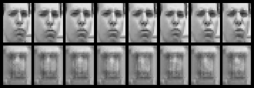
Figure 2 shows the images after the first epoch (epoch 0). The eight images in the first row show the original images from the dataset. And the second row shows the reconstructed images. We can see that the neural network was able to capture very limited number of features from the faces. Most probably it was able to reconstruct the outlines of the eyes and lips. Let’s hope that we get better results further on.

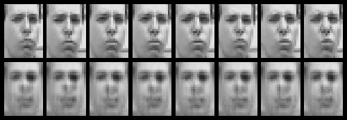
Figure 3 shows the results after 10 epochs. The reconstruction is much better now. The eyes and lips are almost clear. And the neural network is beginning to reconstruct the nose as well.

The above image (figure 4) is from the last epoch. The convolutional neural network is almost able to reconstruct the facial features. Although some features like the nose are still blurry.

Maybe using a neural network with more neurons per layer will help. Or maybe we can use a bigger network with more layers.

Summary and Conclusion

In this post, you got to learn about the about convolutional VAE. You learned how to reconstruct face images using the Frey Face dataset. This tutorial showed a very simple way to work with convolutional VAE and greyscale images. We will work with more complicated colored images in future posts.

If you have any doubts, suggestions, or ideas, then leave them in the comment section. I will surely address them.

You can contact me using the Contact section. You can also find me on LinkedIn, and Twitter.