Implementing Deep Convolutional GAN (DCGAN) with PyTorch

In this tutorial, we will be implementing the Deep Convolutional Generative Adversarial Network architecture (DCGAN). We will go through the paper Unsupervised Representation Learning with Deep Convolutional Generative Adversarial Networks first. This paper by Alec Radford, Luke Metz, and Soumith Chintala was released in 2016 and has become the baseline for many Convolutional GAN architectures in deep learning. We will learn about the DCGAN architecture from the paper. After that, we will implement the paper using PyTorch deep learning framework.

What will you learn in this tutorial?

• You will get to know about the original DCGAN paper.
• We will learn about the architectures of the deep convolutional GAN as described in the paper.
• We will discuss the different parameters/hyperparameters that give the best results while training the DCGAN.
• Then we will implement the DCGAN architecture using the PyTorch deep learning framework.

If you are new to generative adversarial networks in general, then I highly recommend that you go through the previous posts.

• Introduction to Generative Adversarial Networks (GANs).
• Generating MNIST Digit Images using Vanilla GAN with PyTorch.

Going Through the DCGAN Paper

In this section, we will get into some of the details of the DCGAN paper. We will briefly get to know about the architectures, the parameters, and the different datasets used by the authors.

Some of the Important Contributions

Generative adversarial networks (GANs) really began to grow after the famous paper by Goodfellow et al. in 2014. From then till now (the year 2020 at the time writing this tutorial), GANs have made many headlines in the field of deep learning and neural networks. And most of the work has been in the field of computer vision. Now, if we focus on the DCGAN paper here (the year 2016), the following are the contributions from the authors.

• They propose methodologies to train Convolutional GANs in a much stable way.
• The discriminator that emerges after training a DCGAN can be used for image classification tasks. This shows the power of unsupervised training.
• The authors show that the generator can learn to draw specific objects.
• We can also manipulate the semantic properties of the images generated by the generator. This shows that generated vectors have interesting properties.

You will find the above points in detail in the paper itself. We will keep this section brief and move onto the architecture of DCGAN.

The Architecture of DCGAN

The first obvious things we can infer is that the neural network will use convolutional layers. In fact, in the whole DCGAN architecture, there are no fully connected layers.

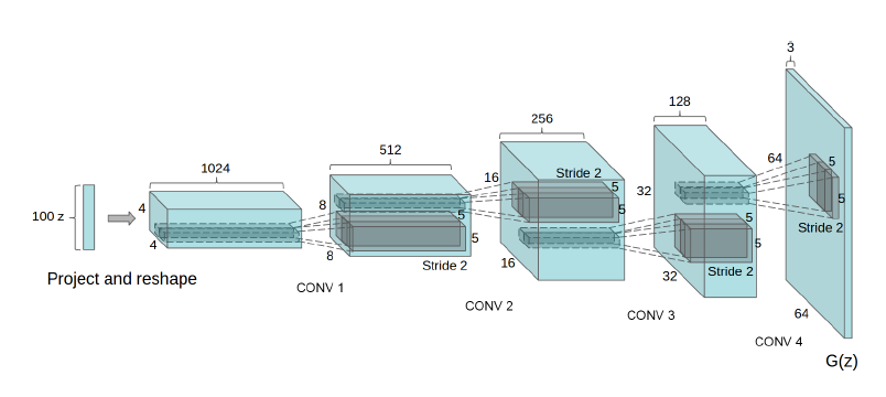
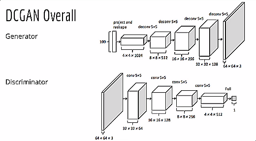
Figure 2 shows the generator network of DCGAN architecture. You can clearly see that there are no fully connected layers. We have only convolutional layers in the network.

Let’s go over the layers step-by-step.

• First, we give the generator a 100-dimensional noise vector as the input. After that, we project and reshape the input.
• Then we have four convolution operations.
• Each time we get an increment in height and width. At the same time, the channels keep on reducing.
• After the first convolution operation, we have 512 output channels. This keeps on reducing with each convolution operation. After the third one, the output channels are 128.
• By the end, we have a generated image of 64×64 dimensions and three output channels.
• Except for the first convolution layer, all the other layers have a stride of 2.

The above points will become even more concrete when we will get into the coding part. Before that, let’s get into some details of the network architecture when building the discriminator and generator networks.

Architectural Details of the DCGAN Model

Remember when we discussed that the authors provide a stable way to train the DCGAN. Well most of it comes down to two things.

• The first one is how we build the discriminator and generator networks.
• The second one comes down to the parameters and hyperparameters.

In this section, we will discuss the architecture of the discriminator and the generator. These guidelines are laid out by the authors of the paper and they work pretty well.

No Max Pooling

DCGAN architecture is a fully convolutional network. This means that we will not use any max-pooling for downsampling. All of the operations will be through strided convolutions only.

Also, the network will not contain any fully connected layers.

Using Batch Normalization

We will use batch normalization while building both, the discriminator and the generator. This mainly tackles two problems in DCGAN and in deep neural networks in general.

• It normalizes the input to each unit of a layer.
• It also helps to deal with poor initialization that may cause problems in gradient flow.

ReLU, LeakyReLU, and Tanh Activations

We will use the ReLU activation function in all the layers of the generator, except for the last one. For the last convolutional layer, we will use Tanh activation function.

For the discriminator, we will use LeakyReLU for all the convolutional layer after applying batch normalization.

The above are the architectural details that the authors have provided in the paper. Applying these successfully while building our DCGAN model will surely help in more stable training.

Hyperparameters to Consider While Training

Now, we will learn about the different parameters and hyperparameters that we can use while training DCGAN. Using the hyperparameter values as provided by the authors will give us the best results while training.

• The very first one is the batch size. The authors used a batch size of 128 for training DCGAN. While implementing the code, will use the same batch size as well.
• We will also carry out weight initialization for the generator and discriminator networks. We will initialize the weights from a zero-centered Normal Distribution with a standard deviation of 0.02.
• As you know, for the discriminator network, we will use the LeakyReLU activation. We will set the slope of the LeakyReLU activation to 0.2.
• We will use the Adam optimizer for training DCGAN. The learning rate of Adam optimizer is going to be 0.0002. The Adam optimizer has a default momentum value \(\beta1\) of 0.9. Instead of 0.9, we will set the value of \(\beta1\) to 0.5. This helps in more stable training and faster convergence.

The above are the hyperparameters that worked best while training DCGAN on the Large-scale Scene Understanding (LSUN), ImageNet-1K, and Faces Dataset. But these hyperparameters should work across most of the deep learning image datasets as well.

Project Structure and the Dataset that We Will Use

We will implement the DCGAN model using the PyTorch deep learning library. There are some other dependencies as well. But if you work with deep learning, you should already have those. If not, just install them as you go through the tutorial.

Coming to the dataset, we will not use any of the datasets that the authors have used for the generative model training. Those datasets range in gigabytes of size. For example, the LSUN Bedroom dataset contains around 3 million images and it is above 3GB in size. It would be highly impractical to train a DCGAN model on such a huge dataset. Instead, we will use the CIFAR10 dataset. The dataset is small in size, has RGB images, and is fairly complex for training a DCGAN model.

PyTorch Framework Version

Note: Currently the code works fine on PyTorch version 1.4.0 (that is torch version 1.4.0 and torchvision version 0.5.0). You will be able to run the code as it is without any errors if you use this version. Newer versions will give give you the following error.

ValueError: Using a target size (torch.Size([128, 1])) that is different to the input size (torch.Size([128])) is deprecated. Please ensure they have the same size.

Try to use PyTorch version 1.4.0 to run the existing error-free.

As training code takes a long time to complete, therefore, I am also linking a Colab link to run the code eaily and error-free. Find the notebook here.

The Project Structure

Now, let’s get down to the project structure. There are many components that we will need to connect. We will not write the whole code in just one python script. It will be highly unreadable and difficult to debug. Instead, we will separate the code into three different scripts. Take a look at the following.

├───input
│   └───data
│       └───cifar-10-batches-py
├───outputs
└───src
    │   dcgan.py
    │   train_dcgan.py
    │   utils.py

• The input folder has a data subfolder that will contain the CIFAR10 dataset. We can use the datasets fucntion of the torchvision module to download the dataset.
• outputs folder will contain the outputs from training the DCGAN model. This includes the generated images, the trained generator weights, and the loss plot as well.
• The src folder has three python scripts.
  • dcgan.py will contain the generator and discriminator network class codes.
  • train_dcgan.py will contain the overall code to train the DCGAN model.
  • And finally, utils.py will contain all the helper and utility functions that will make our work much easier.

We will get into all the details while writing the code. As of now, you make sure that you follow the same structure so that you can easily follow along. I will be telling which code will go into which script in their respective sections.

Now, let’s get into the fun part. That is implementing DCGAN using Python and PyTorch.

Implementing DCGAN using PyTorch

From this section onward, we will be writing the code. There will be many sub-sections so that you can easily know what we are actually doing. As for the python scripts, I will be prompting whenever we will change from one script to another. Also, there will be ample documentation in the code itself. This will help you understand the code much more easily.

Before moving further, I would highly suggest that you use a GPU for training the DCGAN model in this tutorial. Training DCGAN or any GAN model will take a lot of time on CPU. If you do not have a GPU at your disposal, then you should consider Google Colab or Kaggle Kernels for this tutorial.

Implementing the Generator and Discriminator Models

We will begin by writing the code for the generator and discriminator model classes. The code will go into the dcgan.py file. Let’s start with the generator model class.

The Generator Model

Building the model will need just one line of import. We will need the torch.nn module only.

import torch.nn as nn

The next code block will contain the whole generator code. We will get into the explanation after we write the code.

# generator
class Generator(nn.Module):
    def __init__(self, nz):
        super(Generator, self).__init__()
        self.nz = nz
        self.main = nn.Sequential(
            # nz will be the input to the first convolution
            nn.ConvTranspose2d(
                nz, 512, kernel_size=4, 
                stride=1, padding=0, bias=False),
            nn.BatchNorm2d(512),
            nn.ReLU(True),

            nn.ConvTranspose2d(
                512, 256, kernel_size=4, 
                stride=2, padding=1, bias=False),
            nn.BatchNorm2d(256),
            nn.ReLU(True),

            nn.ConvTranspose2d(
                256, 128, kernel_size=4, 
                stride=2, padding=1, bias=False),
            nn.BatchNorm2d(128),
            nn.ReLU(True),

            nn.ConvTranspose2d(
                128, 64, kernel_size=4, 
                stride=2, padding=1, bias=False),
            nn.BatchNorm2d(64),
            nn.ReLU(True),

            nn.ConvTranspose2d(
                64, 3, kernel_size=4, 
                stride=2, padding=1, bias=False),
            nn.Tanh()
        )

    def forward(self, input):
        return self.main(input)

Explanation of the Generator Model Code

• In __init__() function, you will notice that we have the nz parameter. We initialize this as self.nz at line 5. This is the size of the noise vector that the generator will use as the input. You will also see the same in figure 2 which shows the 100-dimensional noise vector as the input to the generator.
• From line 6, we use the Sequential container to build the generator model.
• The size of in_channels for the first convolutional layer is self.nz which is equal to 100. The out_channels is 500 and the kernel size of 4×4. For the first convolutional layer, we have a stride of 1 and a padding of 0. Then we have the batch normalization and the ReLU activation function.
• After that, we have four such convolutional blocks (from line 14 till 36).
• With each subsequent convolution operation, we keep on reducing the output channels. We start from 512 output channels and have 3 output channels after the last convolution operation. 512 => 256 => 128 => 64 => 3. This 3 refers to the three channels (RGB) of the colored images.
• All of the four convolutions have a stride of 2 and a padding of 1 with 4×4 kernel.
• Only the last convolution operation has Tanh activation instead of ReLU. Also, the final image dimension generated by the generator is going to be 64x64x3.
• The forward() function from line 38 makes a forward pass of the noise vector through the generator network. It returns the generated output at line 39.

Note that while building the generator network, we have bias=False for all the layers.

The Discriminator Model

Let’s move on to the discriminator model. The discriminator mode will almost be the reverse of the generator model.

Take a look at the code and you can understand what I am saying.

# discriminator
class Discriminator(nn.Module):
    def __init__(self):
        super(Discriminator, self).__init__()
        self.main = nn.Sequential(
            nn.Conv2d(
                3, 64, kernel_size=4, 
                stride=2, padding=1, bias=False),
            nn.LeakyReLU(0.2, inplace=True),

            nn.Conv2d(
                64, 128, kernel_size=4, 
                stride=2, padding=1, bias=False),
            nn.BatchNorm2d(128),
            nn.LeakyReLU(0.2, inplace=True),

            nn.Conv2d(
                128, 256, kernel_size=4, 
                stride=2, padding=1, bias=False),
            nn.BatchNorm2d(256),
            nn.LeakyReLU(0.2, inplace=True),

            nn.Conv2d(
                256, 512, kernel_size=4, 
                stride=2, padding=1, bias=False),
            nn.BatchNorm2d(512),
            nn.LeakyReLU(0.2, inplace=True),

            nn.Conv2d(
                512, 1, kernel_size=4, 
                stride=1, padding=0, bias=False),
            nn.Sigmoid()
        )

    def forward(self, input):
        return self.main(input)

• We are using the Sequential container just as we did in the case of the generator.
• There are five convolution operations in the discriminator model as well.
• The first convolution operation has three in_channels which corresponds to the three color channels of the CIFAR10 images. The out_channels is 64. The kernel size is 4×4, the stride is 2 and padding is 1. We do not have any batch normalization after the first convolution operation. The LeakyReLU activation has a slope of 0.2, as discussed previously.
• The following three convolution operations are very similar. The output channels keep on increasing till 512 out_channels in the fourth Conv2d(). But we are implementing batch normalization after these three convolution operations.
• The last convolution operation has 1 output channel with Sigmoid activation. This is because we need the discriminator to classify whether an image is real (1) or fake (0). As this is binary classification, therefore, we are using Sigmoid activation. The stride here is 1 and padding is 0.
• The forward() function at line 35 forward passes either the real image or fake image batch through the discriminator network. Then the discriminator returns the binary classifications at line 36.

This is all that we have for the generator and the discriminator model. Take some time to read, analyze, and implement the code by yourself. Eventually, all of this will make sense.

Writing the Code in utils.py File

Now, we will move on to write the code for our utils.py file. These are going to be a few simple but very important functions. In fact, there are going to be five simple functions in the utils.py file. Lets’s get down to writing these.

We will start with importing all the required modules and libraries.

import torch
import torch.nn as nn

from torchvision.utils import save_image

# set the computation device
device = torch.device('cuda' if torch.cuda.is_available() else 'cpu')

The above are all the imports that we need. Along with that we set the computation device at line 7.

All of the following functions contain additional documentation in comment form. That will help you understand the usability even easily.

Functions for Creating Fake and Real Labels

We will start with writing the functions to create the fake and real labels. If you have read my previous article, then you will find this exactly similar to the helper functions in that post.

def label_real(size):
    """
    Fucntion to create real labels (ones)
    :param size: batch size
    :return real label vector
    """
    data = torch.ones(size, 1)
    return data.to(device)

def label_fake(size):
    """
    Fucntion to create fake labels (zeros)
    :param size: batch size
    :returns fake label vector
    """
    data = torch.zeros(size, 1)
    return data.to(device)

• Line 1 defines the label_real() function. This function takes the batch size of the data as input and creates a single-dimensional vector which consists of all ones. For example, if the batch size is 5, then it will return something like the following.
  • [1, 1, 1, 1, 1].
• At line 10, we define the label_fake() function. This is similar to the label_real() function. But this function will return a vector consisting of all zeros equal to the batch size. Something like the following.
  • [0, 0, 0, 0, 0].

Note that, before returning we load the labels on to the computation device. This is really important as the image data and label should have the same computation device.

Function to Create Noise Tensor

Here, we will write the function to create a noise tensor. As you know, the generator will take in a random noise tensor and use it to create the fake images. This following is the function that will create the noise tensor.

def create_noise(sample_size, nz):
    """
    Fucntion to create noise
    :param sample_size: fixed sample size or batch size
    :param nz: latent vector size
    :returns random noise vector
    """
    return torch.randn(sample_size, nz, 1, 1).to(device)

• This function takes two input parameters. One is the sampel_size which is fixed to 64 (we will define it further in this article). The other one is nz which is the dimension of the noise vector. Now, remember that the noise vector is 100 dimensional (figure 2). We will define this later in this article as well.
• So, if you print the size of the noise vector, then you get the following output.
  • [64, 100, 1, 1].

Function to Save the Generator Image Batches

The generator will generate fake images in batches. PyTorch provides the save_image function using which we can easily save the image batches without any further modification. It will handle everything for us.

def save_generator_image(image, path):
    """
    Function to save torch image batches
    :param image: image tensor batch
    :param path: path name to save image
    """
    save_image(image, path, normalize=True)

This function takes two input parameters. The first one is the image batch, and the second one is the image path to save the image.

Function for Weight Initialization

We will need to initialize the weights of the generator and the discriminator from a zero-centered Normal Distribution. We will use a function that will initialize the generator and the discriminator weights. Take a look at the following function.

def weights_init(m):
    """
    This function initializes the model weights randomly from a 
    Normal distribution. This follows the specification from the DCGAN paper.
    https://arxiv.org/pdf/1511.06434.pdf
    Source: https://pytorch.org/tutorials/beginner/dcgan_faces_tutorial.html
    """
    classname = m.__class__.__name__
    if classname.find('Conv') != -1:
        nn.init.normal_(m.weight.data, 0.0, 0.02)
    elif classname.find('BatchNorm') != -1:
        nn.init.normal_(m.weight.data, 1.0, 0.02)
        nn.init.constant_(m.bias.data, 0)

This function is the same as the weight initialization function in this PyTorch tutorial. We will apply the weight initialization to the generator and discriminator after we initialize the networks. We will get into further details when we reach that point.

The above are all the utility functions that we need. From the next section onward, we will move onto write the training code for the generator and discriminator.

Writing the Training Code for the Generator and the Discriminator

Starting from this section, we will write the functions to train the DCGAN model. Along with that we will define all the learning parameters and the hyperparameters as described in the paper. All of the code from here onward will go into train_dcgan.py file.

The following are all the libraries and module that we need to import.

import torch
import torch.nn as nn
import torchvision.transforms as transforms
import torch.optim as optim
import torchvision.datasets as datasets
import numpy as np
import matplotlib

from utils import save_generator_image, weights_init
from utils import label_fake, label_real, create_noise
from dcgan import Generator, Discriminator
from torch.utils.data import DataLoader
from matplotlib import pyplot as plt
from tqdm import tqdm

matplotlib.style.use('ggplot')

Defining all the Learning Parameters and Hyperparameters

Here, we will define all the learning parameters and the hyperparameters according to the paper.

# learning parameters / configurations according to paper
image_size = 64 # we need to resize image to 64x64
batch_size = 128
nz = 100 # latent vector size
beta1 = 0.5 # beta1 value for Adam optimizer
lr = 0.0002 # learning rate according to paper
sample_size = 64 # fixed sample size
epochs = 25 # number of epoch to train

# set the computation device
device = torch.device('cuda' if torch.cuda.is_available() else 'cpu')

• At line 2, we set the image resizing parameter. We will be resizing the image to 64×64 dimension as that is recommended in the paper.
• Line 3 defines the batch size which is equal to 128.
• At line 4 we have nz which is the latent vector (noise vector) size or dimension. The noise vector is going to be 100 dimensional.
• We will use the Adam optimizer for training. The authors recommend to use the beta1 coefficient value as 0.5 instead of the default 0.9. We define that at line 5.
• Line 6 defines the learning rate which is equal to 0.0002.
• The fixed sample size for the noise vector is going to be 64 which we define at line 7.
• At line 8 we define the number of epochs to train for, that is 25.
• Finally, at line 11, we set the computation device.

The above are all the parameters and hyperparameters that we need. All of the hyperparameters values are as per the values that are given in the paper.

Preparing the Dataset

We will use the datasets module from torchvision to download the CIFAR10 dataset. Before downloading the dataset, let’s define the image transforms.

# image transforms
transform = transforms.Compose([
    transforms.Resize(image_size),
    transforms.ToTensor(),
    transforms.Normalize((0.5, 0.5, 0.5), 
    (0.5, 0.5, 0.5)),
])

In the image transforms, we are resizing the image, converting the values to tensors, and normalizing the values as well. The resizing dimensions are 64×64.

Now, we will define the training data and the training data loader. We will just need the training data loader and not the validation data loader. This is because all of the DCGAN operations will happen on the training data only. This includes the fake data generation and the binary classification by the discriminator.

# prepare the data
train_data = datasets.CIFAR10(
    root='../input/data',
    train=True,
    download=True,
    transform=transform
)
train_loader = DataLoader(train_data, batch_size=batch_size, shuffle=True)

Initialize the Generator and Discriminator Networks

Now, we will initialize the generator and discriminator networks.

# initialize models
generator = Generator(nz).to(device)
discriminator = Discriminator().to(device) 

We also need to initialize the weights for the generator and discriminator networks.

# initialize generator weights
generator.apply(weights_init)
# initialize discriminator weights
discriminator.apply(weights_init)

print('##### GENERATOR #####')
print(generator)
print('######################')

print('\n##### DISCRIMINATOR #####')
print(discriminator)
print('######################')

We are applying weight initialization to the generator and discriminator network at lines 2 and 4 respectively. Then, we are also printing both the network architectures at lines 7 and 11.

Defining the Optimizer and Loss Function

Now, we will define the Adam optimizer and loss function.

# optimizers
optim_g = optim.Adam(generator.parameters(), lr=lr, betas=(beta1, 0.999))
optim_d = optim.Adam(discriminator.parameters(), lr=lr, betas=(beta1, 0.999))

# loss function
criterion = nn.BCELoss()

We need two different optimizer initializations. optim_g is the Adam optimizer initialization for the generator network and optim_d is for the discriminator network. Notice that we are applying the beta1 value (0.5) that we have defined previously. The loss function is BCELoss().

Next, we will define two lists.

losses_g = [] # to store generator loss after each epoch
losses_d = [] # to store discriminator loss after each epoch

The losses_g list will store the generator loss after each epoch and the losses_d will store the discriminator loss after each epoch.

Function to Train the Discriminator

In this section, we will write the function to train the discriminator network. If you have gone through my previous article, then you will find it almost the same as the discriminator training function as the one there.

# function to train the discriminator network
def train_discriminator(optimizer, data_real, data_fake):
    b_size = data_real.size(0)
    # get the real label vector
    real_label = label_real(b_size)
    # get the fake label vector
    fake_label = label_fake(b_size)

    optimizer.zero_grad()

    # get the outputs by doing real data forward pass
    output_real = discriminator(data_real).view(-1)
    loss_real = criterion(output_real, real_label)

    # get the outputs by doing fake data forward pass
    output_fake = discriminator(data_fake)
    loss_fake = criterion(output_fake, fake_label)

    # compute gradients of real loss 
    loss_real.backward()
    # compute gradients of fake loss
    loss_fake.backward()
    # update discriminator parameters
    optimizer.step()

    return loss_real + loss_fake

• The function has three input parameters. The discriminator optimizer, the real data, and the fake data.
• First, we get the real labels and fake labels at line 5 and 7 according to the batch size.
• At line 12, we get the outputs by doing a forward pass of the real data through the discriminator. Line 13 calculates the loss for the real outputs and real labels.
• At line 16, we get the outputs from the fake data by doing a forward pass through the discriminator network. And line 17 calculates the loss from the fake outputs and the fake labels.
• Then we compute the gradients of the real and fake losses at lines 20 and 22. We update the parameters and finally return the total loss at line 26.

The above function should not be much confusing. Still, you may take some time to analyze the code.

Function to Train the Generator

Here, we will write the function to train the generator,

# function to train the generator network
def train_generator(optimizer, data_fake):
    b_size = data_fake.size(0)
    # get the real label vector
    real_label = label_real(b_size)

    optimizer.zero_grad()

    # output by doing a forward pass of the fake data through discriminator
    output = discriminator(data_fake)
    loss = criterion(output, real_label)

    # compute gradients of loss
    loss.backward()
    # update generator parameters
    optimizer.step()

    return loss 

• The train_generator() function has only two parameters. One is the generator optimizer and the other one is the fake data (data_fake).
• We get the real labels at line 5.
• Then we forward pass the fake data through the discriminator at line 10 and get the loss values at line 11.
• Then we compute the gradients of the loss and update the generator parameters at line 16.
• Finally, we return the generator loss at line 18.

Train the DCGAN Model for Specified Number of Epochs

Now we are all set to train the DCGAN model for 25 epochs. Before that, let’s create the noise vector that the generator will use to generate the images after each training loop.

# create the noise vector
noise = create_noise(sample_size, nz)

Now, switching the generator and discriminator networks to training mode.

generator.train()
discriminator.train()

We will use a simple for loop to train the generator and discriminator network.

for epoch in range(epochs):
    loss_g = 0.0
    loss_d = 0.0
    for bi, data in tqdm(enumerate(train_loader), total=int(len(train_data)/train_loader.batch_size)):
        image, _ = data
        image = image.to(device)
        b_size = len(image)
        # forward pass through generator to create fake data
        data_fake = generator(create_noise(b_size, nz)).detach()
        data_real = image
        loss_d += train_discriminator(optim_d, data_real, data_fake)
        data_fake = generator(create_noise(b_size, nz))
        loss_g += train_generator(optim_g, data_fake)

    # final forward pass through generator to create fake data...
    # ...after training for current epoch
    generated_img = generator(noise).cpu().detach()
    # save the generated torch tensor models to disk
    save_generator_image(generated_img, f"../outputs/gen_img{epoch}.png")
    epoch_loss_g = loss_g / bi # total generator loss for the epoch
    epoch_loss_d = loss_d / bi # total discriminator loss for the epoch
    losses_g.append(epoch_loss_g)
    losses_d.append(epoch_loss_d)

    print(f"Epoch {epoch+1} of {epochs}")
    print(f"Generator loss: {epoch_loss_g:.8f}, Discriminator loss: {epoch_loss_d:.8f}")

• We define loss_g and loss_d to keep track of the batch-wise loss values of the generator and discriminator respectively.
• Starting from line 4, we iterate through the batches in one epoch of training data.
• Line 9 creates the fake data from the generator. We use this fake data for discriminator and generator training at line 11 and 13.
• At line 17 the generator creates the fake data after training completes for the current epoch. This is the image that we save to disk at line 19.
• We calculate the epoch-wise losses at lines 20 and 21. Then we append them to losses_g and losses_d at lines 22 and 23.

Saving the Generator Weights and Plotting the Loss Graph

As the training is complete now, we can save the final generator weights.

print('DONE TRAINING')
# save the model weights to disk
torch.save(generator.state_dict(), '../outputs/generator.pth')

Finally, we just need to plot and save the loss graph to disk.

# plot and save the generator and discriminator loss
plt.figure()
plt.plot(losses_g, label='Generator loss')
plt.plot(losses_d, label='Discriminator Loss')
plt.legend()
plt.savefig('../outputs/loss.png')
plt.show()

This marks the end of writing all the code that we need for training the DCGAN model. If you find any section confusing, then I recommend going through the paper a bit to get a better understanding.

Running the train_dcgan.py File

To train the DCGAN model on the CIFAR10 data, we just need to run the train_dcgan.py file. Open up your terminal and cd into the src folder in the project directory. From there type the following command.

python train_dcgan.py

The following is the truncated output.

##### GENERATOR #####
Generator(
  (main): Sequential(
    (0): ConvTranspose2d(100, 512, kernel_size=(4, 4), stride=(1, 1), bias=False)
    (1): BatchNorm2d(512, eps=1e-05, momentum=0.1, affine=True, track_running_stats=True)
    (2): ReLU(inplace=True)
    (3): ConvTranspose2d(512, 256, kernel_size=(4, 4), stride=(2, 2), padding=(1, 1), bias=False)
    (4): BatchNorm2d(256, eps=1e-05, momentum=0.1, affine=True, track_running_stats=True)
    (5): ReLU(inplace=True)
    (6): ConvTranspose2d(256, 128, kernel_size=(4, 4), stride=(2, 2), padding=(1, 1), bias=False)
    (7): BatchNorm2d(128, eps=1e-05, momentum=0.1, affine=True, track_running_stats=True)
    (8): ReLU(inplace=True)
    (9): ConvTranspose2d(128, 64, kernel_size=(4, 4), stride=(2, 2), padding=(1, 1), bias=False)
    (10): BatchNorm2d(64, eps=1e-05, momentum=0.1, affine=True, track_running_stats=True)
    (11): ReLU(inplace=True)
    (12): ConvTranspose2d(64, 3, kernel_size=(4, 4), stride=(2, 2), padding=(1, 1), bias=False)
    (13): Tanh()
  )
...
Epoch 1 of 25
Generator loss: 7.95222950, Discriminator loss: 0.47085580
391it [03:06,  2.10it/s]
...
Epoch 24 of 25
Generator loss: 2.81237388, Discriminator loss: 0.66299611
391it [03:23,  1.92it/s]
Epoch 25 of 25
Generator loss: 3.44565058, Discriminator loss: 0.57825148
DONE TRAINING

I again strongly advise that you use either Google Colab or Kaggle Kernel if your system does not have a dedicated Nvidia GPU. Else the code may take a few hours to run.

In general, 25 epochs may not be enough for getting good results on the CIFAR10 dataset. If you are using Colab or Kaggle, then you may run for more epochs. But for the sake of easier reproducibility, I have included the results after training for 25 epochs.

Analyzing the Outputs

Finally, we get to see how our model has performed after training for 25 epochs. The following is the loss graph plot that we have saved to the disk.

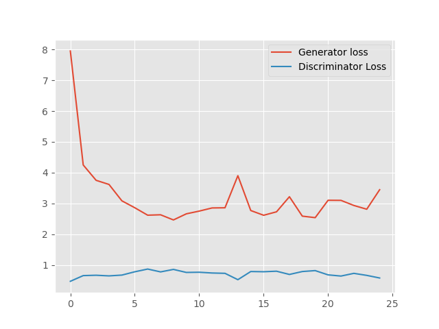
Figure 3 shows that the generator loss started quite high, around 8. While the discriminator loss was low, around 0.47. This is expected as in the beginning the generator cannot produce very good fake images. Therefore, the discriminator can easily classify them. As training progresses, the generator loss starts to reduce to anything between 2.5 and 3. Around this time, the discriminator loss increases as it is not longer able to classify the fake images with high probability.

We can see that after 23 epochs, the discriminator loss is again starting to decrease. Maybe it is starting to learn to distinguish between the generated fake images and real images. Only training for longer will reveal further results. Do give it a try on your own.

The Generated Images

Now, let’s take a look at the images that are generated by the generator.

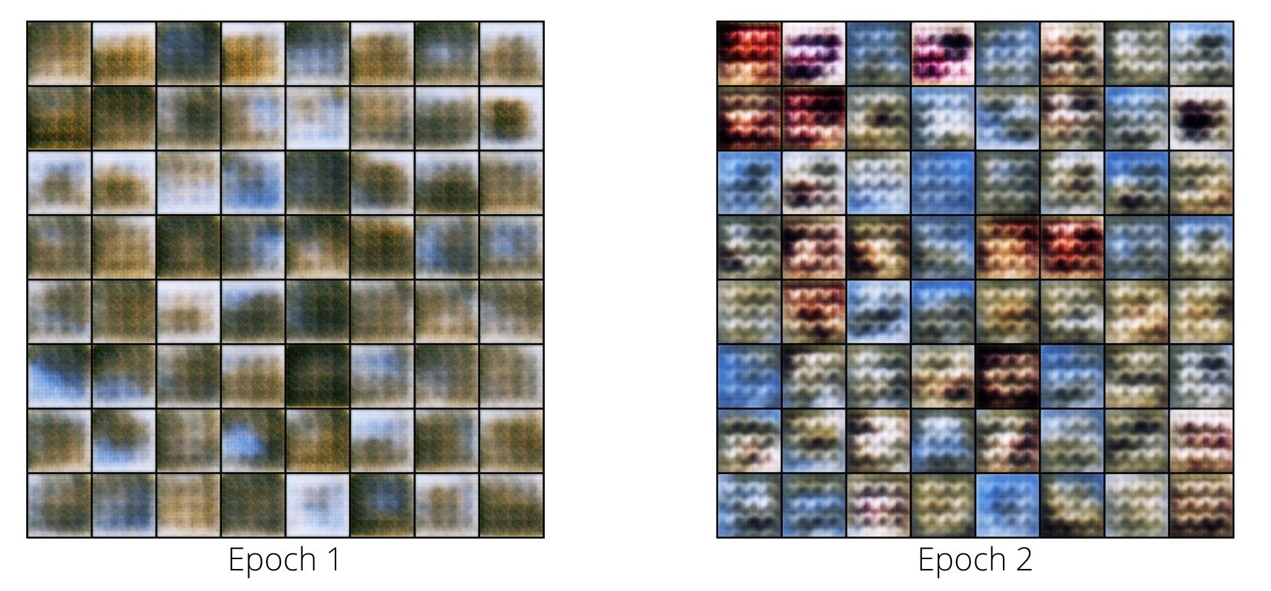
Figure 4 shows the generated images from epoch 1 and 2. We can see that they are just random noise. Although it seems that the generator has learned to generate some good colors by the end of second epoch.

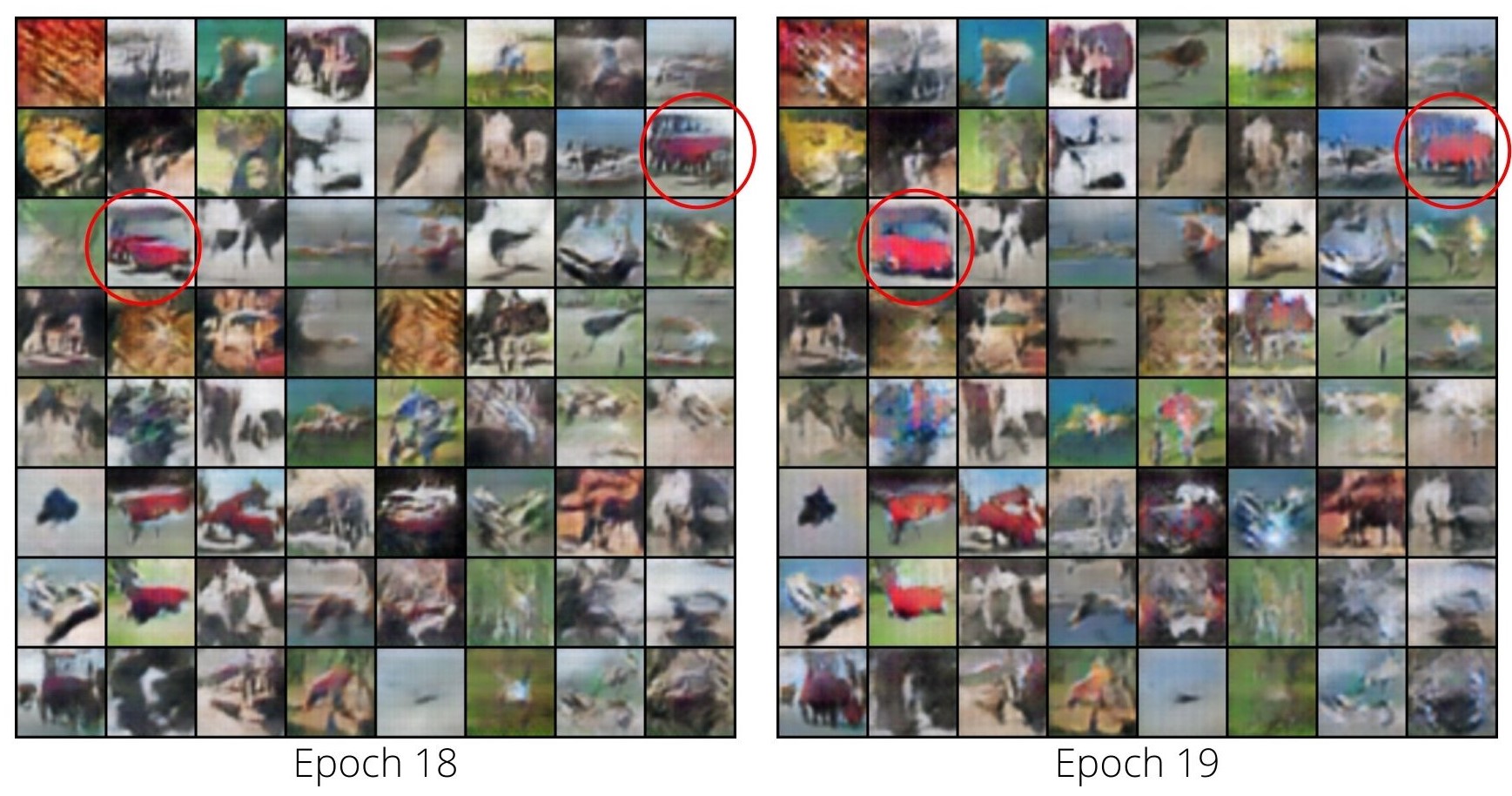
In figure 5, the results looks a bit better. It seems that the generator is learning some useful patterns. Most probably, it is learning to generate the automobile images from the CIFAR10 dataset. I have marked the grids in red circle, where it seems that the generator has generated automobile images.

And finally, the following figure shows the generated images from the final epoch (epoch 25).

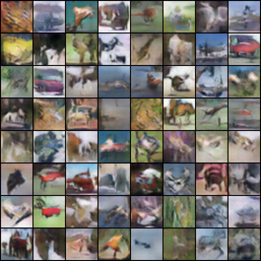
You can see that the results here are worse. It also tells us why the generator loss was higher in the final epoch. That was because it did not produce very good results in the final epoch.

A Bit of Bonus Content

Here, I am including a Colab notebook where you will find the code to this post. You can easily run this in your browser with GPU computing in case you do not have a dedicated GPU.

Link to Colab notebook.

Summary and Conclusion

In this post, you learned how to implement Deep Convolutional Generative Adversarial Network using PyTorch on the CIFAR10 dataset. You got to learn about the different hyperparameters and parameters that produce the best results and also had hands-on experience with coding the DCGAN model.

I hope that you learned a lot from this tutorial. If you have any doubts, thoughts, or suggestions, then please use the comment section to post them. I will surely address them.

You can contact me using the Contact section. You can also find me on LinkedIn, and Twitter.