Automatic Mixed Precision Training for Deep Learning using PyTorch

In this tutorial, we will learn about Automatic Mixed Precision Training (AMP) for deep learning using PyTorch. At the time of writing this, the stable version of PyTorch 1.6 has been released. And with that, we have the native support for Automatic Mixed Precision training for deep learning models.

You may have a lot of questions about the what, why, and how by reading the title of this tutorial. Maybe the most important question here is, will you benefit by going through this tutorial? The short and simple answer is yes, for sure. And you will benefit more if PyTorch is the deep learning framework that you work with. Even if you work with other frameworks like TensorFlow, then also you will able to learn and apply the concepts there (transfer learning!). After all, only the syntax will be a bit different.

So, what will you learn after going through this tutorial?

• What is Automatic Mixed Precision training in deep learning?
• Its effects and benefits when using large models and datasets in deep learning training.
• All the NVIDIA GPUs that support AMP training.
• Syntax and PyTorch code to use AMP for deep learning training.
• Using ResNet50 and transfer learning training to compare FP32 and AMP training.

I hope that the above points excite you enough to move ahead with this tutorial. And don’t worry if you do not have an Nvidia GPU in your system. You will still be able the experience the benefits through the code.

Introduction to Automatic Mixed Precision Training in Deep Learning

In deep learning, all the training and gradient operations happen using 32-bit floating-point operations. We can call these FP32 operations as well. But we can achieve the same amount of accuracy as FP32 by using half the floating-point operations. That is, we can also use FP16 (16-bit floating-point operations) to achieve the same amount of accuracy with many other benefits as well.

So, basically speaking, using AMP training instead of single-precision FP32, will benefit us in the following ways.

• Training deep learning models.
• In operations that involve gradient operations like backpropagation and updating the parameters.

Native AMP support from PyTorch 1.6 also replaces Apex. Apex is a PyTorch tool to use Mixed-Precision training easily.

We will get into the details of the above benefits and a few more very soon.

The best part is that you will be able to use AMP with just a few lines of code. You can also use AMP for existing deep learning codes that have not used AMP before. Of course, you will need to install PyTorch 1.6 for that, but that is a very small issue.

Will AMP Affect Accuracy?

One of the questions that come to mind is, does using FP16 instead of FP32 not affect the accuracy adversely? The answer is no, it will not. We will be able to get the same, if not more accurate results by using FP16 training instead of FP32 training. We will cover all these details while getting into the benchmark details of AMP.

Benefits of using Automatic Mixed Precision Training for Deep Learning

In this section, we will get into all benefits and also the performance benchmarks of using AMP for deep learning training.

Mixed Precision Training Accuracy on the NVIDIA A100 GPU

The benchmarks that we will see here are from training a ResNet50 deep learning model. To compare the results of FP16 and FP32, the training has been carried out for the same number of epochs but with different floating precision.

Take a look at the table below.

epochs	Mixed Precision Top 1(%)	TF32 Top1(%)
90	76.93	76.85

We can see in table 1 that mixed-precision training has a slightly better accuracy after 90 epochs. Although that is not the point here. The important thing is that we are able to get just as good of a performance from FP16 training. The A100 GPUs are based on the Ampere architecture and contain tensor cores which greatly help in deep learning training.

Similarly, the following table shows the training accuracy at different epochs.

epochs	Mixed Precision Top 1(%)	FP32 Top1(%)
50	76.25	76.26
90	77.09	77.01
250	78.42	78.30

Table 2 clearly shows that not just the final convergence epochs but also the intermediate epochs have very similar accuracy when training with FP16. This shows that FP16 can clearly replace FP32 training.

Performance Speedup While using Mixed Precision Training

Not just the training accuracy, we can also get a huge boost in reducing training times when using mixed precision training for deep learning.

On a V100 GPU, we can expect a speedup of 1.5x to 5.5x depending upon the deep learning model.

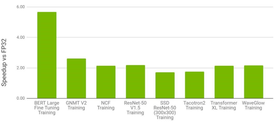
Figure 2 shows the training speedup while using mixed precision training on 8x NVIDIA V100 GPUs. V100 GPUs are based on the Volta architecture which contains tensor cores just like the A100 GPUs. Now, you may ask, “Why are we discussing the GPU models and architectures? Is it not enough to know that we are training models using AMP?” Apparently, in the world of deep learning, hardware now plays a very important role. And it is very important to know which GPU models and architectures provide what features. It is even more important if you want to build a system for deep learning and want to get the best results.

We will bring the performance benchmarks to an end here. You can read more about it here. Rather, we will move on to some other benefits that we ourselves can experience hands-on.

Benefits of Automatic Mixed Precision for Deep Learning Training

In this section, we will discuss the benefits of using mixed-precision training that we will be able to experience while training our models. Let’s dive into the details.

Speedup in Linear and Convolution Layer Operations

If you are a deep learning practitioner or do deep learning projects regularly, then you know that the more layers, the larger the model, and the longer it takes to train it.

But we can reduce the training time significantly by using mixed-precision. This is especially true for models with linear and convolution layers. These layers contain a lot of mathematical operations which greatly benefit from the half-precision computation of FP16.

Speedup in Memory-Limited Operations

Using FP16 also speeds up many memory-limited operations. This is because we need to access just half the bytes of memory of what we need with single-precision (FP32).

Reduction in Memory Requirements

This is perhaps the benefit of using mixed-precision that we can experience very easily.

Using mixed-precision reduces the memory requirement to a great extent. So much so that we can use larger models, and larger mini batches while training our model. Even if we do not have tensor cores available in our GPU, still we will be able to gain speedup from using larger mini batches.

From my own experience, I was able to use literally double the batch-size when training deep learning models with mixed-precision as compared to training with single-precision. In fact, this is exactly what will be experiencing further on in this article.

NVIDIA Architectures needed for Automatic Mixed Precision Training

In this section, there will be some good news and some bad news but good news mostly.

According to NVIDIA, to get the full array of benefits of mixed-precision training, we need a GPU based on one of the following architectures.

• Ampere.
  • A100 line of GPUs.
  • The upcoming 30 series GPU. Likes of RTX 3080.
• Turing.
  • NVidia T4.
  • The RTX 20 series of GPUs.
• Volta.
  • The V100 line of GPUs.

The reason that NVIDIA emphasizes having one of the above GPUs is that they have tensor cores. And tensor cores help a lot in deep learning and with mixed-precision training as well.

Now, I perfectly understand that you may not have these GPUs in your system. And if you are a student you may not have access to a GPU or may have a GTX GPU, or at most have an RTX 20 series GPU (lucky you). I myself have a GTX 1060 GPU and still was able to use some features of mixed-precision training. This means that you can too while following this tutorial. And you do not need to have even a GTX GPU on your system, let alone one with tensor cores.

If you have an RTX GPU or a GPU with tensor cores, then you may directly jump to the coding section of this tutorial.

And if you do not have access to a GPU or have GTX 10 series GPU, then follow along with the next section.

NVIDIA Pascal Architecture and Mixed Precision Training

Let’s keep this short.

NVIDIA GTX 10 series GPUs (1050, 1060, 1070, and 1080) are all based on the Pascal architecture. They do not contain tensor cores obviously but they do support 16-bit floating-point operations. So, you are good to go even if you have a GTX 10 series GPU.

Now, what if you do not have a GPU in your system? Well, if you are a deep learning/machine learning person, then you must know about Kaggle. Kaggle provides notebooks where we have access to a GPU. That GPU is the Tesla P100 GPU (at the time of writing this) and it is based on Pascal architecture as well. So, even if you do not have a GPU, you will still be able to experience the benefits of mixed precision training if you follow along with this tutorial.

In this tutorial, with the Pascal architecture, we will able to get the following benefits of mixed-precision training.

• We can train larger models while requiring less memory.
• We can train models with larger minibatches.

The above two should provide us enough plus points to consider mixed-precision training over single-precision training.

We had enough discussion on the technical hardware stuff. And since we know that we will able to use mixed-precision training, let’s get down to the code that will enable us to do so.

PyTorch Code to Use Mixed Precision Training

Before doing anything, we first need to install PyTorch 1.6 on our system. Head over here and choose your preferred method to install PyTorch 1.6 on your system.

Using Mixed-Precision Training with PyTorch

To get the benefits of mixed-precision training, we need to learn about two things.

• Autocasting.
• Gradient Scaling.

Autocasting

Autocasting, when enabled, automatically uses float16 data type (FP16) for all those operations that support it. To know about all the operations that support FP16 take a look at this. For now, it is enough to know that linear layers and convolutional layers support FP16 operations.

To use autocasting, we need to use the torch.cuda.amp.autocast() package. Now, it is very important to know that, autocasting should only be used for wrapping the forward pass of the network and the loss computation. The syntax will look something like this.

# enable autocasting for forward pass
with torch.cuda.amp.autocast():
    # calculate outputs and loss within the autocast block
    outputs = model(data)
    loss = criterion(outputs, target)

The story does not end here. If we use FP16 operations for the forward pass, we also need to take care of some other things for the backward pass. This is where Gradient Scaling comes into play.

Gradient Scaling

When we use autocasting, some operations in the forward pass have float16 inputs. This means that the backward pass for those operations will also produce float16 gradients. These float16 gradients with small magnitude may face the problem of underflow. This will result in the loss of the gradient update while doing the backward pass. So, how do we prevent this underflow?

We can use gradient scaling which multiplies the loss values by a scale factor. Now the backward pass will happen on these scaled losses instead of the original loss values. This will also cause the gradients to scale when the backpropagation takes place. And since they have a larger magnitude now, underflow will not occur.

The above may sound complicated but it is just three lines of code actually. First, we need to initialize the gradient scaler by using the following syntax. Take a look at the following.

scaler = torch.cuda.amp.GradScaler() 

# scale the loss and do backprop
scaler.scale(loss).backward()

# update the scaled parameters
scaler.step(optimizer)

# update the scaler for next iteration
scaler.update()

By looking at the above block, you may realize that there is just one extra line of code. That is updating the scaler. The previous two lines of code replace the conventional loss.backward() and optimizer.step() lines.

Combining Autocasting and Gradient Scaling in a Training Iteration

Let’s take look at how autocasting and gradient scaling work in a training iteration.

import torch 
# initialize gradient scaler
scaler = torch.cuda.amp.GradScaler() 
 
for data, label in data_iter: 
    optimizer.zero_grad() 
    # enable autocasting for mixed precision
    with torch.cuda.amp.autocast(): 
        outputs = model(data)
        loss = model(data) 
 
    # scale the loss and do backprop
    scaler.scale(loss).backward()

    # update the scaled parameters
    scaler.step(optimizer)

    # update the scaler for next iteration
    scaler.update()

This is all we need to do for mixed-precision training instead of single-precision training. I think that it is easier than you expected it would be.

Next, we will write the code that will train a deep learning model with mixed-precision.

ResNet-50 Transfer Learning on Caltech-256 Dataset

From this section onward, we will begin to write the code that will enable us to realize the benefits of mixed-precision training over single-precision training.

Just one more thing. We will not be going into a detailed explanation of all the codes in this section. I will explain all those code parts that contain AMP code but not the other code parts. The main reason is, we want to learn how to apply mixed-precision training in deep learning. If you need to learn more about PyTorch and deep learning, then you may take look at all the posts that I have.

Some Prerequisites Before Getting into the Code

There are a few things that we need to take care of before we move into the coding details.

The Project Structure and Dataset

If you are following along with your own computer, then it is better if you have the following directory structure for this tutorial. This will ensure that you can follow along smoothly. Also, we will be using the Caltech-256 dataset in this tutorial. Go ahead and download the dataset from here.

Once it is downloaded, just rename the ZIP file as Caltech256. It will allow for easier path insertion while coding.

And the following is the project directory structure.

───input
│   └───Caltech256
│       └───256_ObjectCategories
│           ├───001.ak47
│           ├───002.american-flag
...
├───outputs
└───src
    │   dataset.py
    │   engine.py
    │   model.py
    │   preprocess.py
    │   train.py

• Extract the Caltech256 folder inside the input folder. This contains another subfolder, that is 256_ObjectCategories which contains all the images inside their respective folders according to the class names.
• The outputs folder will contain all the outputs training the deep learning model will produce. This will include the graphical plots for loss and accuracy and the trained model.
• Inside the src folder we have five python scripts. We will get into the details of the content while writing the code.

Install PyTorch 1.6

The next step is to install PyTorch version 1.6 if you have not done so already. You can install it by following the instructions and choosing your preferences here.

Now make sure that you are creating either a new Anaconda environment or a new Python virtualenv, whichever you use. This will ensure that your old PyTorch and its other related packages do not conflict with the new one.

Install Albumentations

The next step is to install an image augmentation library, which is albumentations. You can install it using pip.

pip install albumentations

Install PyTorch Pretrained Models

Finally, we need to install PyTorch pretrained models from here. Install it by using the following command.

pip install pretrainedmodels

This GitHub repository has a number of pretrained ConvNets for PyTorch, some of which include: NASNet, ResNeXt, ResNet, InceptionV4, InceptionResnetV2, Xception, DPN.

Writing the Code For Mixed-Precision Training

If you want to move ahead while coding on your own system, then follow along.

And if you do not have a GPU at your disposal or have one that does not support AMP or simply want another alternative, then this is the link to a Kaggle Notebook for the same.

Caltech-256 AMP PyTorch.

Writing the Code to Preprocess the Data and Create a data.csv File

We will start with the preprocess.py script. This script will preprocess our dataset and create a new CSV file that will contain all the image paths and the targets as numerical labels.

import os
import pandas as pd
import numpy as np

from tqdm import tqdm
from sklearn.preprocessing import LabelBinarizer

root_dir = '../input/Caltech256/256_ObjectCategories'
# get all the folder paths
all_paths = os.listdir(root_dir)

# create a DataFrame
data = pd.DataFrame()

images = []
labels = []
counter = 0
for folder_path in tqdm(all_paths, total=len(all_paths)):
    # get all the image names in the particular folder
    image_paths = os.listdir(f"{root_dir}/{folder_path}")
    # get the folder as label
    label = folder_path.split('.')[-1]
    
    if label == 'clutter':
        continue

    # save image paths in the DataFrame
    for image_path in image_paths:
        if image_path.split('.')[-1] == 'jpg':
            data.loc[counter, 'image_path'] = f"{root_dir}/{folder_path}/{image_path}"
            labels.append(label)
            counter += 1

labels = np.array(labels)
# one-hot encode the labels
lb = LabelBinarizer()
labels = lb.fit_transform(labels)

# add the image labels to the dataframe
for i in range(len(labels)):
    index = np.argmax(labels[i])
    data.loc[i, 'target'] = int(index)
    
# shuffle the dataset
data = data.sample(frac=1).reset_index(drop=True)

print(f"Number of labels or classes: {len(lb.classes_)}")
print(f"The first one hot encoded labels: {labels[0]}")
print(f"Mapping the first one hot encoded label to its category: {lb.classes_[0]}")
print(f"Total instances: {len(data)}")
 
# save as CSV file
data.to_csv('../input/data.csv', index=False)
 
print(data.head(5))

We will not go into the detailed explanation of the above code, so take a moment to analyze it. You can execute it by:

python preprocess.py

This will create a data.csv inside the input folder which looks something like this.

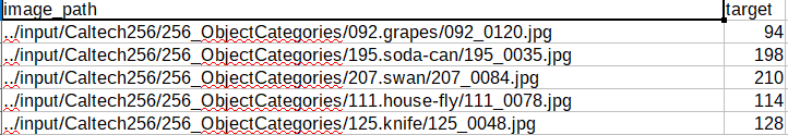
Figure 3 shows the first few cells of the data.csv file. This contains the image paths and the corresponding labels according to the image category.

Preparing the Dataset

The next step is to read the images and prepare the dataset (image and labels) as torch tensors.

All of the code here will go into the dataset.py file.

import albumentations
import numpy as np
import torch

from PIL import Image
from torch.utils.data import Dataset

# custom dataset
class ImageDataset(Dataset):
    def __init__(self, images, labels=None, tfms=None):
        self.X = images
        self.y = labels

        # apply augmentations
        if tfms == 0: # if validating
            self.aug = albumentations.Compose([
                albumentations.Resize(224, 224, always_apply=True),
            ])
        else: # if training
            self.aug = albumentations.Compose([
                albumentations.Resize(224, 224, always_apply=True),
                albumentations.HorizontalFlip(p=0.5),
                albumentations.ShiftScaleRotate(
                    shift_limit=0.3,
                    scale_limit=0.3,
                    rotate_limit=15,
                    p=0.5
                ),
            ])
         
    def __len__(self):
        return (len(self.X))
    
    def __getitem__(self, i):
        image = Image.open(self.X[i])
        image = image.convert('RGB')
        image = self.aug(image=np.array(image))['image']
        image = np.transpose(image, (2, 0, 1)).astype(np.float32)
        label = self.y[i]
        return {
            'image': torch.tensor(image, dtype=torch.float), 
            'target': torch.tensor(label, dtype=torch.long)
        }

The above script returns the images and labels as torch tensors (lines 40 to 43).

Preparing the Neural Network Model

As discussed before, we will use the ResNet50 neural network for transfer learning. The following code will go into the model.py file.

import pretrainedmodels
import torch.nn as nn
import torch.nn.functional as F

class ResNet50(nn.Module):
    def __init__(self, pretrained, requires_grad):
        super(ResNet50, self).__init__()
        if pretrained is True:
            self.model = pretrainedmodels.__dict__['resnet50'](pretrained='imagenet')
        else:
            self.model = pretrainedmodels.__dict__['resnet50'](pretrained=None)
            
        if requires_grad == True:
            for param in self.model.parameters():
                param.requires_grad = True
        elif requires_grad == False:
            for param in self.model.parameters():
                param.requires_grad = False
        
        self.l0 = nn.Linear(2048, 256)

    def forward(self, x):
        batch, _, _, _ = x.shape
        x = self.model.features(x)
        x = F.adaptive_avg_pool2d(x, 1).reshape(batch, -1)
        l0 = self.l0(x)
        return l0

model = ResNet50(pretrained=True, requires_grad=False)
# print(model)

We are changing the last linear layer at line 20 so that the output features match the total number of classes, which is 256.

Writing the Training and Validation Functions

This section is really important. We will write the training and validation functions here. We write the code that will use mixed-precision while training and validation.

Let’s first write the code, then we will get down to the explanation. The following code will go into the engine.py file.

from tqdm import tqdm

import torch

# training function
def fit(model, dataloader, optimizer, criterion, train_data, device, use_amp):
    print('Training')
    if use_amp == 'yes':
        scaler = torch.cuda.amp.GradScaler() 

    model.train()
    train_running_loss = 0.0
    train_running_correct = 0
    for i, data in tqdm(enumerate(dataloader), total=int(len(train_data)/dataloader.batch_size)):
        data, target = data['image'].to(device), data['target'].to(device)
        optimizer.zero_grad()
        
        if use_amp == 'yes':
            with torch.cuda.amp.autocast():
                outputs = model(data)
                loss = criterion(outputs, target)
        
        elif use_amp == 'no':
            outputs = model(data)
            loss = criterion(outputs, target)
            
        train_running_loss += loss.item()
        _, preds = torch.max(outputs.data, 1)
        train_running_correct += (preds == target).sum().item()
        
        if use_amp == 'yes':
            scaler.scale(loss).backward()
            scaler.step(optimizer)
            scaler.update()
        
        elif use_amp == 'no':
            loss.backward()
            optimizer.step()
        
    train_loss = train_running_loss/len(dataloader.dataset)
    train_accuracy = 100. * train_running_correct/len(dataloader.dataset)    
    return train_loss, train_accuracy

# validation function
def validate(model, dataloader, optimizer, criterion, val_data, device, use_amp):
    print('Validating')
    if use_amp == True:
        scaler = torch.cuda.amp.GradScaler() 
        
    model.eval()
    val_running_loss = 0.0
    val_running_correct = 0
    with torch.no_grad():
        for i, data in tqdm(enumerate(dataloader), total=int(len(val_data)/dataloader.batch_size)):
            data, target = data['image'].to(device), data['target'].to(device)
            
            if use_amp == 'yes':
                with torch.cuda.amp.autocast():
                    outputs = model(data)
                    loss = criterion(outputs, target)
        
            elif use_amp == 'no':
                outputs = model(data)
                loss = criterion(outputs, target)
            
            val_running_loss += loss.item()
            _, preds = torch.max(outputs.data, 1)
            val_running_correct += (preds == target).sum().item()
        
        val_loss = val_running_loss/len(dataloader.dataset)
        val_accuracy = 100. * val_running_correct/len(dataloader.dataset)        
        return val_loss, val_accuracy

Explanation of the Above Code Block

Let’s start with the training function, that is fit().

• One of the input parameters of fit() is use_amp. This is going to be a string, the value can either be yes or no. If the value is yes, then we will use mixed-precision for training. If it is no, then we will continue with the regular training.
• First of all, we initialize the gradient scaler at line 9 of use_amp is yes.
• If use_amp is yes, then we will enable autocasting for the forward pass. Take a look at lines 18 to 21. If it is no, then we will not use autocasting (lines 23 to 25).
• Similarly for the backpropagation, if use_amp is yes, then we will scale the loss, update the scaled parameters, and update the scaler. Else, we continue with the conventional backpropagation (lines 36 to 38).

We take the same approach for the validate() function, except we need not backpropagate the loss.

I hope that the above code is understandable. We just need to change a few lines of code if we are using mixed-precision for training.

Writing the Code for train.py File

To train our model with or without mixed-precision, we will have to execute the fit() and validate() functions. We write the code for that inside the train.py file.

"""
Usage:
> python train.py --batch-size 256 --use-amp no
> python train.py --batch-size 512 --use-amp no # batch size of 512 will OOM error without AMP on GTX 1060
> python train.py --batch-size 512 --use-amp yes
"""

from sklearn.model_selection import train_test_split
from model import model
from dataset import ImageDataset
from torch.utils.data import DataLoader
from engine import fit, validate

import torch.optim as optim
import time
import torch.nn as nn
import argparse
import pandas as pd
import matplotlib
import torch 
import matplotlib.pyplot as plt

# build and parse the argument parser
parser = argparse.ArgumentParser()
parser.add_argument('-b', '--batch-size', dest='batch_size', type=int, 
                    help='batch size for the dataset', default=512)
parser.add_argument('-a', '--use-amp', dest='use_amp', 
                    help='to use Automatic Mixed Precision or not',
                    default='yes', choices=['yes', 'no'])
args = vars(parser.parse_args())

# learning parameters
batch_size = args['batch_size']
print(f"Batch size: {batch_size}")
epochs = 10
lr = 0.0001
use_amp = args['use_amp']
print(f"Use AMP: {use_amp}")

# computation device
device = torch.device('cuda' if torch.cuda.is_available() else 'cpu')

# get the dataset ready
df = pd.read_csv('../input/data.csv')
X = df.image_path.values # image paths
y = df.target.values # targets
(xtrain, xtest, ytrain, ytest) = train_test_split(X, y,
	test_size=0.10, random_state=42)
print(f"Training instances: {len(xtrain)}")
print(f"Validation instances: {len(xtest)}")
train_data = ImageDataset(xtrain, ytrain, tfms=1)
test_data = ImageDataset(xtest, ytest, tfms=0)
# dataloaders
train_data_loader = DataLoader(train_data, batch_size=batch_size, shuffle=True)
valid_data_loader = DataLoader(test_data, batch_size=batch_size, shuffle=False)

# model
model.to(device)
# optimizer
optimizer = optim.Adam(model.parameters(), lr=lr)
# loss function
criterion = nn.CrossEntropyLoss()
# total parameters and trainable parameters
total_params = sum(p.numel() for p in model.parameters())
print(f"{total_params:,} total parameters.")
total_trainable_params = sum(
    p.numel() for p in model.parameters() if p.requires_grad)
print(f"{total_trainable_params:,} trainable parameters.")

train_loss , train_accuracy = [], []
val_loss , val_accuracy = [], []
if use_amp == 'yes':
    print('Tranining and validating with Automatic Mixed Precision')
elif use_amp == 'no':
    print('Tranining and validating without Automatic Mixed Precision')
    
start = time.time()
for epoch in range(epochs):
    print(f"Epoch {epoch+1} of {epochs}")
    train_epoch_loss, train_epoch_accuracy = fit(model, train_data_loader, 
                                                 optimizer, criterion, 
                                                 train_data, device, use_amp)
    val_epoch_loss, val_epoch_accuracy = validate(model, valid_data_loader, 
                                                 optimizer, criterion, 
                                                 test_data, device, use_amp)
    train_loss.append(train_epoch_loss)
    train_accuracy.append(train_epoch_accuracy)
    val_loss.append(val_epoch_loss)
    val_accuracy.append(val_epoch_accuracy)
    print(f"Train Loss: {train_epoch_loss:.4f}, Train Acc: {train_epoch_accuracy:.2f}")
    print(f'Val Loss: {val_epoch_loss:.4f}, Val Acc: {val_epoch_accuracy:.2f}')
end = time.time()

print(f"Took {((end-start)/60):.3f} minutes to train for {epochs} epochs")
    
# save model checkpoint
torch.save({
            'epoch': epochs,
            'model_state_dict': model.state_dict(),
            'optimizer_state_dict': optimizer.state_dict(),
            'loss': criterion,
            }, f"../outputs/amp_{use_amp}_model.pth")

# accuracy plots
plt.figure(figsize=(10, 7))
plt.plot(train_accuracy, color='green', label='train accuracy')
plt.plot(val_accuracy, color='blue', label='validataion accuracy')
plt.xlabel('Epochs')
plt.ylabel('Accuracy')
plt.legend()
plt.savefig(f"../outputs/amp_{use_amp}_accuracy.png")
plt.show()
 
# loss plots
plt.figure(figsize=(10, 7))
plt.plot(train_loss, color='orange', label='train loss')
plt.plot(val_loss, color='red', label='validataion loss')
plt.xlabel('Epochs')
plt.ylabel('Loss')
plt.legend()
plt.savefig(f"../outputs/amp_{use_amp}_loss.png")
plt.show()

Explanation of the Above Code Block

At the top I have provided the execution commands with different parameters and batch sizes.

For the argument parser, we have the batch size and whether to use AMP or not (from lines 24 to 30). We are using the use-amp argument while calling the fit() and validate() functions.

Starting from line 97, we are saving the trained models weights also and the accuracy and loss graphical plots.

You will find all of the code in this Kaggle Notebook as well. The only difference is the batch size as we have access to 16GB of VRAM in Kaggle Notebooks.

Now, let’s move on to execute and train the model.

Note that if you have a different GPU with more or less memory than mine (GTX 1060 with 6GB VRAM), then you may increase and decrease the batch size accordingly.

Training with 256 Batch Size and No Automatic Mixed Precision

We will start with executing the code with 256 batch size and without using any mixed-precision for training. Head over to the src folder in your terminal and type the following command.

python train.py --batch-size 256 --use-amp no

You should see output similar to the following.

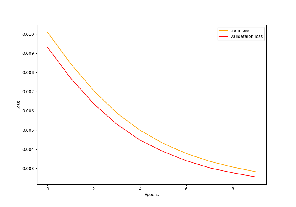
Batch size: 256
Use AMP: no
Training instances: 26802
Validation instances: 2978
26,081,576 total parameters.
524,544 trainable parameters.
Tranining and validating without Automatic Mixed Precision
Epoch 1 of 10
Training
105it [21:42, 12.41s/it]
Validating
12it [01:56,  9.70s/it]
Train Loss: 0.0191, Train Acc: 9.65
Val Loss: 0.0168, Val Acc: 26.63
...
Epoch 10 of 10
Training
105it [04:33,  2.61s/it]
Validating
12it [00:26,  2.18s/it]
Train Loss: 0.0042, Train Acc: 81.81
Val Loss: 0.0039, Val Acc: 83.11
Took 68.051 minutes to train for 10 epochs

We are training for 10 epochs. A batch size of 256 with ResNet50 transfer learning occupies around 3.9GB of my 6GB GTX 1060 VRAM. By the end of the last epoch, we have 83.11% validation accuracy and 0.0039 validation loss.

Let’s take a look at the saved plots.

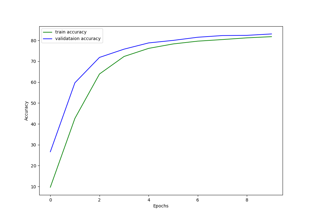
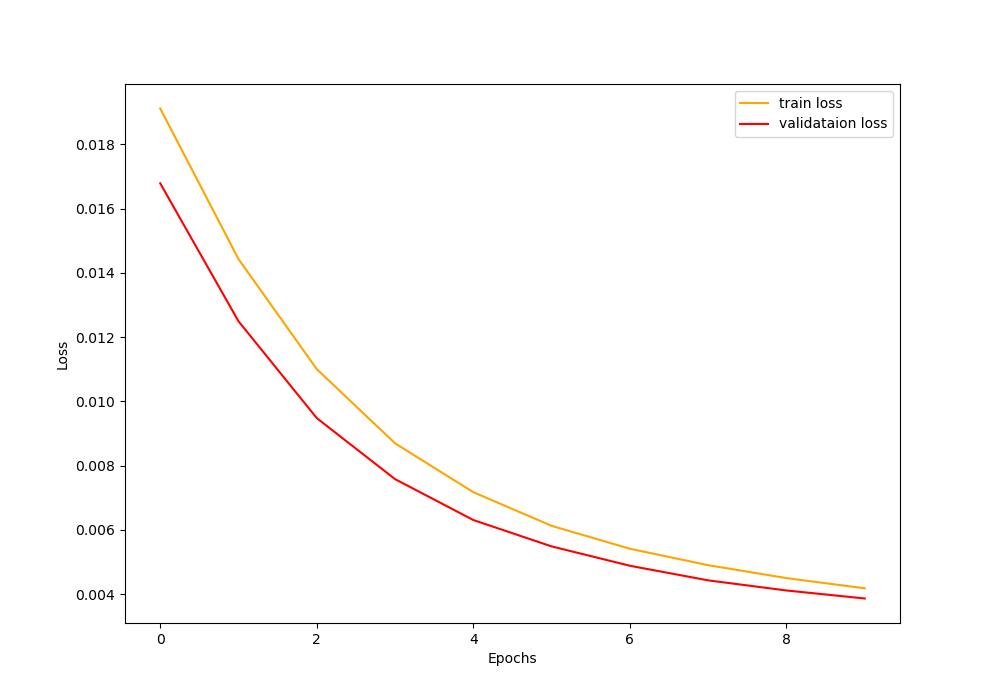
Figure 4 and figure 5 show the accuracy and loss graphs respectively.

Also note that with 256 batch size and without AMP, the total training time is a little over 68 minutes. We will see how much of a training time we gain when using larger batch sizes with AMP.

Training with 512 Batch Size and No AMP

Now, let’s try to train with 512 batch size but without using AMP.

python train.py --batch-size 512 --use-amp no

The gives the following OOM (Out Of Memory) error.

RuntimeError: CUDA out of memory. Tried to allocate 1.53 GiB (GPU 0; 6.00 GiB total capacity; 2.30 GiB already allocated; 1.09 GiB free; 3.46 GiB reserved in total by PyTorch)

Simply, we cannot use such large batch size with 6GB of VRAM.

Now, let’s see what we can achieve when using mixed-precision for training.

Training with 512 Batch Size and Using AMP

It is time to see whether using AMP for training allows us to use such large batch sizes or not.

To train with mixed-precision and a batch size of 512, use the following command.

python train.py --batch-size 512 --use-amp yes

If everything goes well, then you will see output similar to the following.

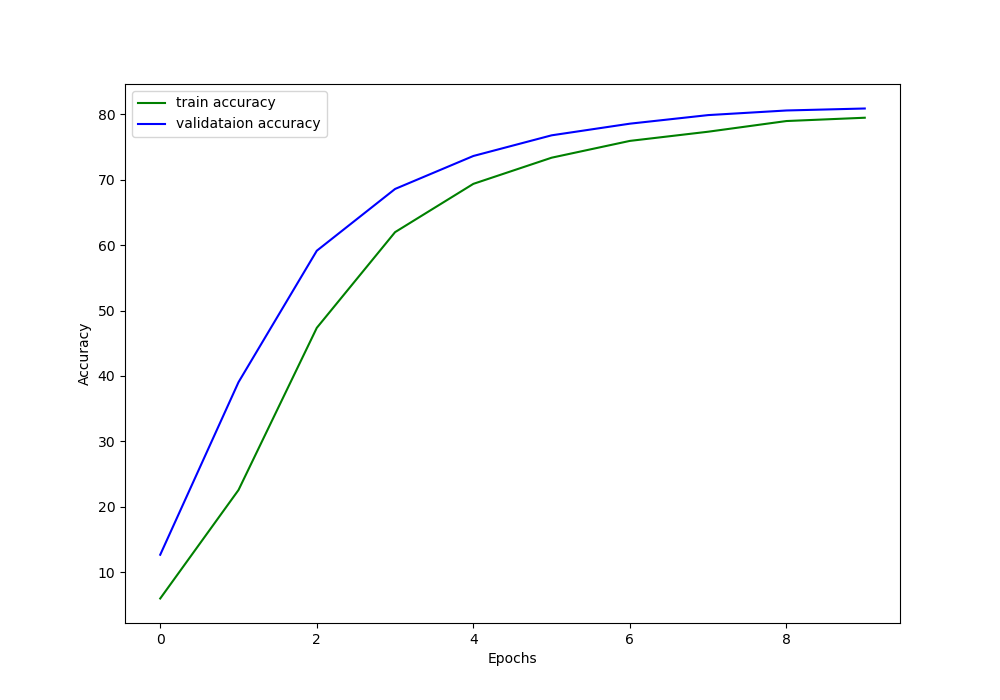
Batch size: 512
Use AMP: yes
Training instances: 26802
Validation instances: 2978
26,081,576 total parameters.
524,544 trainable parameters.
Tranining and validating with Automatic Mixed Precision
Epoch 1 of 10
Training
53it [19:32, 22.13s/it]
Validating
6it [01:56, 19.37s/it]
Train Loss: 0.0101, Train Acc: 6.01
Val Loss: 0.0093, Val Acc: 12.69
...
Epoch 10 of 10
Training
53it [03:56,  4.46s/it]
Validating
6it [00:23,  3.92s/it]
Train Loss: 0.0028, Train Acc: 79.45
Val Loss: 0.0026, Val Acc: 80.86
Took 61.672 minutes to train for 10 epochs

The code ran successfully. In this my VRAM memory usage around 4GB. We can literally use double the batch size with mixed-precision training compared to what we can with single-precision training.

The final loss is 0.0026 which is less than the loss that we got from without mixed-precision training. Although the accuracy is a bit lower, I think that we can easily solve that by using a random seed.

Also, take a look at the total training time. It is almost 7 minutes less than the previous one. Now imagine the gains that we will achieve with more training epochs. And if you have Tensor Cores in your GPU, then the gains will be even higher.

The following two figures show the accuracy and loss graphical plots.

We will wrap this article here. I think that now you are well equipped with trying to play around with AMP and training your own deep learning models as well.

Summary and Conclusion

In this tutorial, you learned about Automatic Mixed Precision and how to use mixed-precision for training deep neural networks. You also got to know about the benefits of mixed-precision training like:

• Being able to train larger models.
• With larger bath sizes.
• And less training time.

If you have any thoughts, doubts, or suggestions, then leave them in the comment section. I will surely address them.

You can contact me using the Contact section. You can also find me on LinkedIn, and Twitter.