Lane Detection using Mask RCNN - An Instance Segmentation Approach

Jump to Download Code

Lane detection and segmentation have a lot of use cases, especially in self-driving vehicles. With lane detection and segmentation, the vehicle gets to see different types of lanes. This allows it to accordingly plan the route and action. Of course, there are several other components involved along with computer vision and deep learning. But this serves as the first step. In this article, we will try to solve the first step involving computer vision and deep learning. We will train a Mask RCNN model for lane detection and segmentation. We are taking an instance segmentation approach to detect and segment various types of lane lines.

Figure 1. A sample output showing lane detection and segmentation using Mask RCNN.

Solving lane detection and segmentation can be a challenging task, even with a powerful model like Mask RCNN. This is because almost every image or frame involves very thin objects (lane lines) which are also far away. But we will try our best to optimize the model as much as possible and get the best results for lane detection using instance segmentation.

Before we move any further, let’s take a look at the points that we will cover in this post:

We will start with a discussion of the lane detection and segmentation dataset.
Next, we will talk about the Mask RCNN instance segmentation model and why we choose it.
Moving forward, we will discuss the training scripts and code files.
After training the model, we will analyze the results and run inference on images and videos.
We will finish the article with a discussion of how to improve the project even further.

The Lane Detection and Segmentation Dataset

The lane detection dataset that we will train the Mask RCNN model on is originally available on Roboflow. But we will use a slightly modified version that I have prepared. You can find the road lane instance segmentation dataset on Kaggle.

The dataset contains 1021 training samples and 112 test samples.

There are 6 object classes in total. They are:

divider-line
dotted-line
double-line
random-line
road-sign-line
solid-line

You can go ahead, download, and extract the dataset locally. After extracting the dataset, you will find the following structure:

road_lane_instance_segmentation
├── annotations
│   ├── instances_train2017.json
│   └── instances_val2017.json
├── train2017 [1021 entries exceeds filelimit, not opening dir]
├── val2017 [112 entries exceeds filelimit, not opening dir]
├── README.dataset.txt
└── README.roboflow.txt

The modified version on Kaggle has JSON annotation format just like the COCO object detection dataset. The training and validation folders are named train2017 and val2017 respectively. Similarly, the annotations folder contains instances_train2017.json and instances_val2017.json. Other than that, there are a few text files from the original Roboflow dataset.

Visualizing Dataset Samples

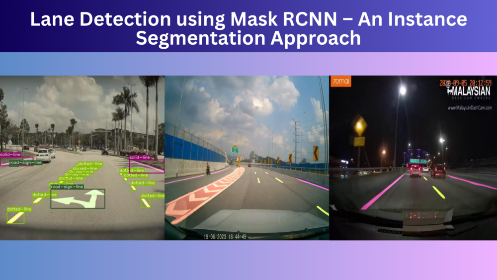
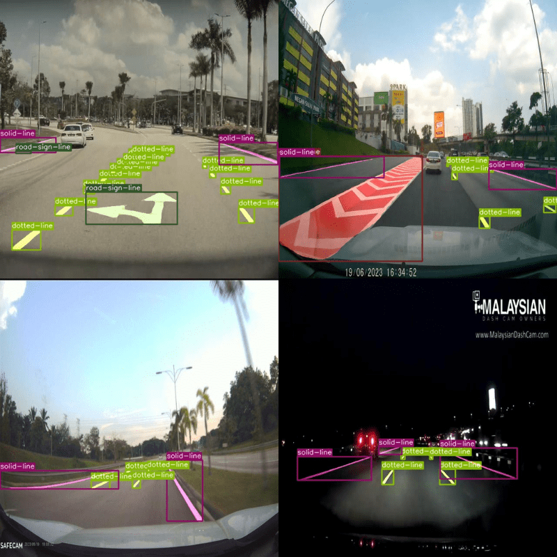
Let’s take a look at a few samples from the dataset.

Figure 2. Ground truth sample 1 from the lane detection and segmentation dataset.

Figure 3. Ground truth sample 2 from the lane detection and segmentation dataset.

Figure 4. Ground truth sample 3 from the lane detection and segmentation dataset.

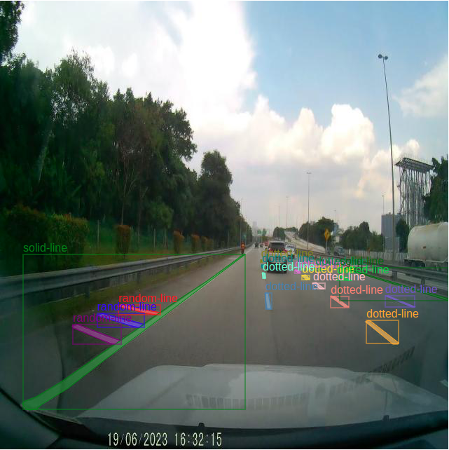
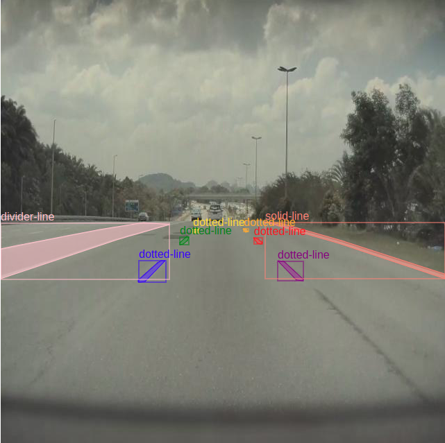
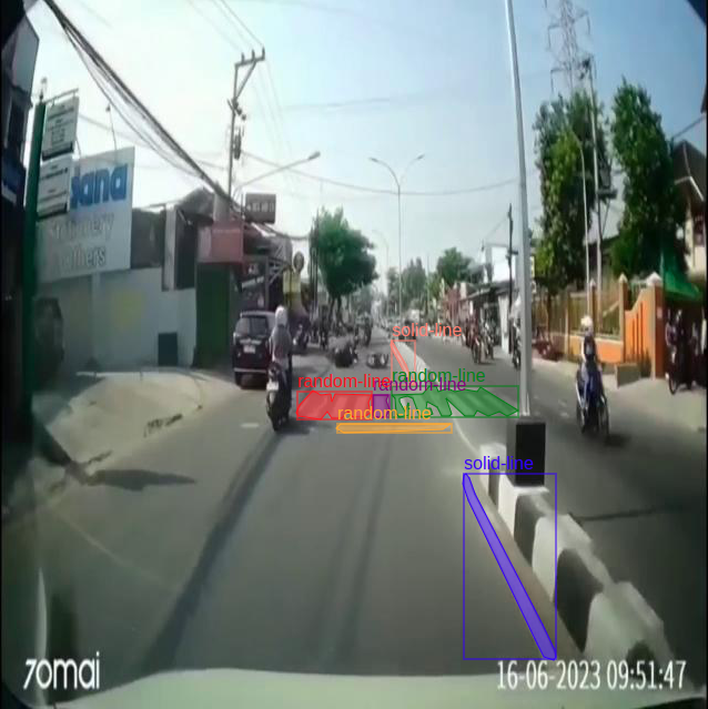
The above figures show a few samples with the annotations from the dataset. We can see almost all the images are driving dashcam videos taken from real footage. So, the model will always get to see real-world data while training.

However, it is very important to note that some of the classes in the dataset are heavily underrepresented. These include categories like double-line and road-sign-line. So, the model may not get trained optimally for each class.

We will end the discussion of the dataset here. Feel free to explore it a bit on your own before moving forward.

The Project Directory Structure

Here is the complete project directory structure.

├── input
│   ├── inference_data
│   └── road_lane_instance_segmentation
├── metrics
│   ├── coco_eval.py
│   ├── coco_utils.py
│   └── utils.py
├── notebooks
│   └── visualize.ipynb
├── outputs
│   ├── inference
│   └── training
├── class_names.py
├── custom_utils.py
├── engine.py
├── group_by_aspect_ratio.py
├── inference_image.py
├── inference_video.py
├── infer_utils.py
├── presets.py
├── train.py
└── transforms.py

The road_lane_instance_segmentation dataset directory resides inside the input directory. It also contains an inference_data directory with a few videos from the internet on which we will carry out inference.
The notebooks directory contains a notebook to visualize the ground truth data.
Inside the outputs directory, we have all the training and inference outputs within their respective subdirectories.
We have a lot of Python files directly inside the parent project directory. These include the training and inference scripts among others. Also, the metrics directory contains the code for the evaluation using pycocotools.

All the code files, trained weights, and inference data will be available via the download section in this article. If you wish to carry out training, please download the dataset from Kaggle and arrange it in the above structure.

PyTorch Version and Other Dependencies

The codebase for this article uses PyTorch 2.0.1 on Ubuntu 20.04. I recommend using at least PyToch 2.0.0 to get the best performance.

Also, we will use pycocotools for evaluation. If you are on any of the supported Linux OS, you can install it using the following command.

pip install pycocotools

There are other requirements for visualizations and inference which you can install as you move along.

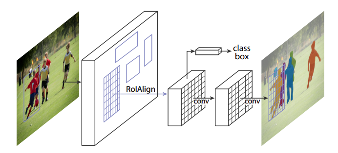
The Mask RCNN Model for Instance Segmentation

The Mask RCNN instance segmentation model is still one of the best models out there till now for instance segmentation.

With the release of Mask RCNN ResNet50 FPN V2 we have even better pretrained weights. The new model provides mask mAP of 41.8% and box mAP of 47.4%. Further, this model has been trained with a new recipe which makes it even more robust when fine-tuning Mask RCNN on a new dataset. The new recipe includes post-paper optimizations which improve the mAP by 9.5% for boxes and 7.2% for masks.

The Mask RCNN framework for instance segmentation. — Figure 5. The Mask RCNN framework for instance segmentation (**source**).

However, one downside of the newer model is that it uses heavier RPN, box, and mask heads. This makes the model slower compared to its previous version. For the time being, we will still move forward with the better and slower version and check its performance while training.

That said, we will still observe the inference speed (FPS) on videos at the end.

All training and inference experiments were carried out on a machine with 10 GB RTX 3080 GPU, 10th generation i7 CPU, and 32 GB of RAM.

Download Code

Download the Source Code for this Tutorial

Lane Detection and Segmentation using PyTorch Mask RCNN

The codebase for this article is quite large. So, we will not discuss all the code files. Rather, we will take a very practical approach and discuss what methods we use to train the best Mask RCNN model that we can.

We will be adapting code from the Torchvision repository and modifying it according to our needs.

Dataset Preparation and Data Augmentation

Dataset preparation and data augmentation are some of the most important steps for any deep learning project. Although most of the dataset preparation steps are handled by the scripts that we will use, we still have a good amount of control over the data augmentation that we want to apply.

From experiments, I found that applying some advanced augmentations allows us to train for longer without overfitting and also reach higher metrics for object detection and segmentation as well.

The transforms.py file contains a lot of augmentation techniques. Among these, we have two powerful data augmentation techniques for object detection and instance segmentation. They are:

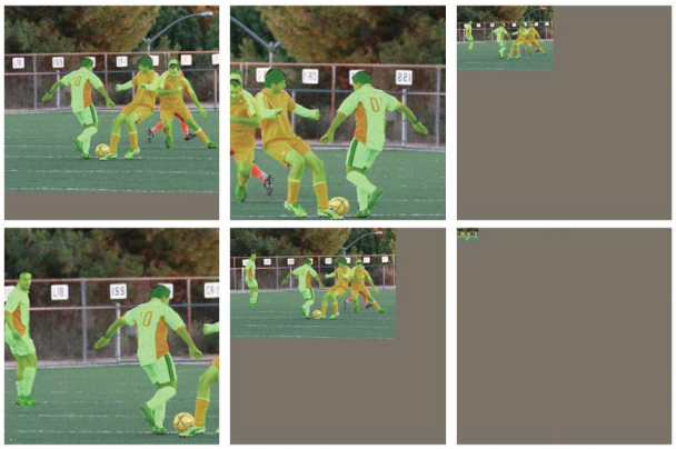
LSJ (Large Scale Jittering)
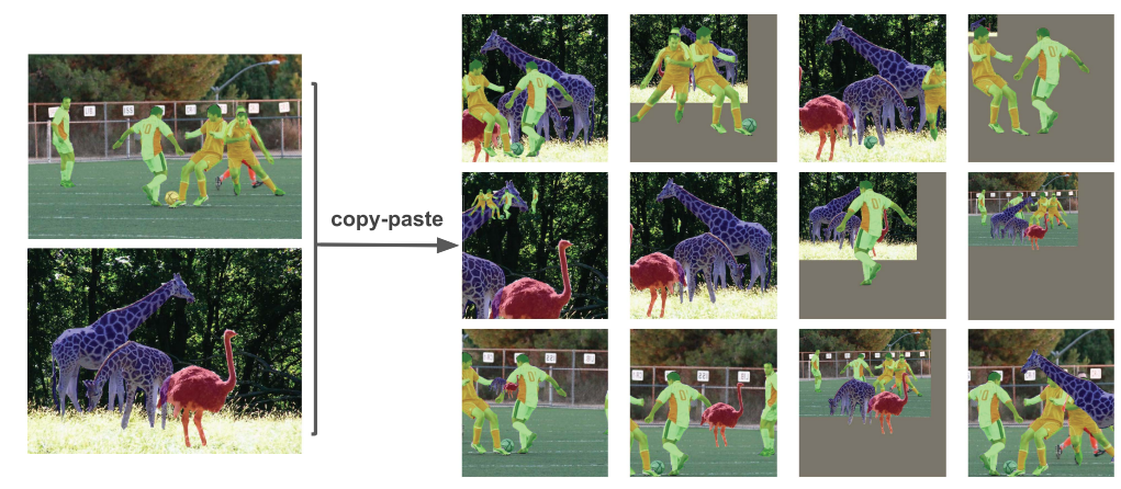
Simple Copy-Paste

The above augmentations were introduced in the paper Simple Copy-Paste is a Strong Data Augmentation Method for Instance Segmentation.

LSJ resizes the images from a range of 0.1 to 2.0 scale which allows the model to learn features of both small and large objects.

Large scale jittering data augmentation. — Figure 6. Large scale jittering data augmentation (**source**).

Simple Copy-Paste copies and pastes objects (instances) from one image into another. This allows the model to see diverse images which it may not encounter directly from the dataset distribution.

Simple copy-paste data augmentation. — Figure 7. Simple copy-paste data augmentation (**source**).

As we can see, applying the above augmentations will surely help us train a much more robust model. Moving forward, we will see how to apply these augmentations when executing the training script.

Other Helpful Scripts

Before moving to the training script, here are some other Python files that you may want to take a look at.

engine.py: This file contains the training and validation functions. The validation function calls pycocotools for evaluation to provide the mAP (Mean Average Precision) for object detection and segmentation.
presets.py: This file includes all the dataset augmentations presets that we can apply during training. We will be applying the lsj dataset augmentation technique.
custom_utils.py: It contains a simple function to plot the mAP graphs after each epoch.

Note: A lot of files from the original Torchvision repository have been slightly modified to make our work easier along the way. As we move along with future posts, the scripts may be updated and provided along with that post through the download section.

The Training Script

The train.py file is the executable script that we will run from the command line. It has a lot of command line arguments. But we will focus only on those that we will use while executing the script.

The training script saves a separate model weight file after each epoch and the checkpoint of every epoch by the name of checkpoint.pth.

Let’s start the training and see how Mask RCNN performs on the lane detection dataset. We can execute the following command from the project’s root directory to start the training.

python train.py \
--data-path input/road_lane_instance_segmentation \
--model maskrcnn_resnet50_fpn_v2 \
--weights MaskRCNN_ResNet50_FPN_V2_Weights.COCO_V1 \
--batch-size 4 \
--epochs 20 \
--lr 0.005 \
--output-dir outputs/training/road_line \
--amp \
--lr-steps 10 \
--data-augmentation lsj \
--use-copypaste

Following are the details of the command line arguments that we use in the above command:

--data-path: This accepts the directory path where the dataset is present in the COCO format.
--model: The model that we want to use. Here, we are using the Mask RCNN ResNet50 FPN V2 model.
--weights: The weights enum. To match the above model, we are providing the appropriate weight file name.
--batch-size: This is the batch size that we want to use for the data loaders. Here, it is 4. It uses around 8.5 GB of VRAM. Please reduce the batch size in case you face OOM (Out Of Memory) error.
--epochs: The number of epochs to train for. We are training for 20 epochs.
--lr: The base learning rate after the initial warm-up.
--output-dir: This is the directory name where all the model checkpoints and mAP graphs will be saved. It will be created automatically if not present.
--amp: A boolean argument indicating that we want to use Automatic Mixed Precision.
--lr-steps: Number of epochs after which to apply the step learning rate scheduler.
--data-augmentation: As we discussed earlier, we are applying the lsj data augmentation here.
--use-copypaste: A boolean argument indicating that we want to use the Simple Copy-Paste augmentation.

Note: We can use the Simple Copy-Paste augmentation only if --data-augmentation is lsj.

Analyzing the Results

These are the results from the command line from the last few epochs.

.
.
.
Epoch: [15] Total time: 0:01:31 (0.3610 s / it)
Test:  [  0/112]  eta: 0:00:22  model_time: 0.0498 (0.0498)  evaluator_time: 0.0106 (0.0106)  time: 0.1983  data: 0.1369  max mem: 5146
Test:  [100/112]  eta: 0:00:00  model_time: 0.0508 (0.0521)  evaluator_time: 0.0177 (0.0211)  time: 0.0744  data: 0.0018  max mem: 5146
Test:  [111/112]  eta: 0:00:00  model_time: 0.0450 (0.0521)  evaluator_time: 0.0150 (0.0210)  time: 0.0706  data: 0.0018  max mem: 5146
Test: Total time: 0:00:08 (0.0782 s / it)
Averaged stats: model_time: 0.0450 (0.0521)  evaluator_time: 0.0150 (0.0210)
Accumulating evaluation results...
DONE (t=0.05s).
Accumulating evaluation results...
DONE (t=0.04s).
IoU metric: bbox
 Average Precision  (AP) @[ IoU=0.50:0.95 | area=   all | maxDets=100 ] = 0.564
 Average Precision  (AP) @[ IoU=0.50      | area=   all | maxDets=100 ] = 0.794
 Average Precision  (AP) @[ IoU=0.75      | area=   all | maxDets=100 ] = 0.616
 Average Precision  (AP) @[ IoU=0.50:0.95 | area= small | maxDets=100 ] = 0.258
 Average Precision  (AP) @[ IoU=0.50:0.95 | area=medium | maxDets=100 ] = 0.655
 Average Precision  (AP) @[ IoU=0.50:0.95 | area= large | maxDets=100 ] = 0.775
 Average Recall     (AR) @[ IoU=0.50:0.95 | area=   all | maxDets=  1 ] = 0.370
 Average Recall     (AR) @[ IoU=0.50:0.95 | area=   all | maxDets= 10 ] = 0.625
 Average Recall     (AR) @[ IoU=0.50:0.95 | area=   all | maxDets=100 ] = 0.640
 Average Recall     (AR) @[ IoU=0.50:0.95 | area= small | maxDets=100 ] = 0.348
 Average Recall     (AR) @[ IoU=0.50:0.95 | area=medium | maxDets=100 ] = 0.762
 Average Recall     (AR) @[ IoU=0.50:0.95 | area= large | maxDets=100 ] = 0.810
IoU metric: segm
 Average Precision  (AP) @[ IoU=0.50:0.95 | area=   all | maxDets=100 ] = 0.397
 Average Precision  (AP) @[ IoU=0.50      | area=   all | maxDets=100 ] = 0.752
 Average Precision  (AP) @[ IoU=0.75      | area=   all | maxDets=100 ] = 0.405
 Average Precision  (AP) @[ IoU=0.50:0.95 | area= small | maxDets=100 ] = 0.133
 Average Precision  (AP) @[ IoU=0.50:0.95 | area=medium | maxDets=100 ] = 0.510
 Average Precision  (AP) @[ IoU=0.50:0.95 | area= large | maxDets=100 ] = 0.613
 Average Recall     (AR) @[ IoU=0.50:0.95 | area=   all | maxDets=  1 ] = 0.279
 Average Recall     (AR) @[ IoU=0.50:0.95 | area=   all | maxDets= 10 ] = 0.464
 Average Recall     (AR) @[ IoU=0.50:0.95 | area=   all | maxDets=100 ] = 0.477
 Average Recall     (AR) @[ IoU=0.50:0.95 | area= small | maxDets=100 ] = 0.230
 Average Recall     (AR) @[ IoU=0.50:0.95 | area=medium | maxDets=100 ] = 0.622
 Average Recall     (AR) @[ IoU=0.50:0.95 | area= large | maxDets=100 ] = 0.626
.
.
.
Epoch: [19] Total time: 0:01:32 (0.3627 s / it)
Test:  [  0/112]  eta: 0:00:22  model_time: 0.0504 (0.0504)  evaluator_time: 0.0114 (0.0114)  time: 0.2033  data: 0.1404  max mem: 5146
Test:  [100/112]  eta: 0:00:00  model_time: 0.0515 (0.0539)  evaluator_time: 0.0166 (0.0216)  time: 0.0781  data: 0.0018  max mem: 5146
Test:  [111/112]  eta: 0:00:00  model_time: 0.0456 (0.0539)  evaluator_time: 0.0157 (0.0215)  time: 0.0724  data: 0.0018  max mem: 5146
Test: Total time: 0:00:09 (0.0807 s / it)
Averaged stats: model_time: 0.0456 (0.0539)  evaluator_time: 0.0157 (0.0215)
Accumulating evaluation results...
DONE (t=0.05s).
Accumulating evaluation results...
DONE (t=0.06s).
IoU metric: bbox
 Average Precision  (AP) @[ IoU=0.50:0.95 | area=   all | maxDets=100 ] = 0.538
 Average Precision  (AP) @[ IoU=0.50      | area=   all | maxDets=100 ] = 0.778
 Average Precision  (AP) @[ IoU=0.75      | area=   all | maxDets=100 ] = 0.573
 Average Precision  (AP) @[ IoU=0.50:0.95 | area= small | maxDets=100 ] = 0.243
 Average Precision  (AP) @[ IoU=0.50:0.95 | area=medium | maxDets=100 ] = 0.660
 Average Precision  (AP) @[ IoU=0.50:0.95 | area= large | maxDets=100 ] = 0.773
 Average Recall     (AR) @[ IoU=0.50:0.95 | area=   all | maxDets=  1 ] = 0.363
 Average Recall     (AR) @[ IoU=0.50:0.95 | area=   all | maxDets= 10 ] = 0.613
 Average Recall     (AR) @[ IoU=0.50:0.95 | area=   all | maxDets=100 ] = 0.628
 Average Recall     (AR) @[ IoU=0.50:0.95 | area= small | maxDets=100 ] = 0.334
 Average Recall     (AR) @[ IoU=0.50:0.95 | area=medium | maxDets=100 ] = 0.768
 Average Recall     (AR) @[ IoU=0.50:0.95 | area= large | maxDets=100 ] = 0.818
IoU metric: segm
 Average Precision  (AP) @[ IoU=0.50:0.95 | area=   all | maxDets=100 ] = 0.386
 Average Precision  (AP) @[ IoU=0.50      | area=   all | maxDets=100 ] = 0.733
 Average Precision  (AP) @[ IoU=0.75      | area=   all | maxDets=100 ] = 0.394
 Average Precision  (AP) @[ IoU=0.50:0.95 | area= small | maxDets=100 ] = 0.133
 Average Precision  (AP) @[ IoU=0.50:0.95 | area=medium | maxDets=100 ] = 0.498
 Average Precision  (AP) @[ IoU=0.50:0.95 | area= large | maxDets=100 ] = 0.613
 Average Recall     (AR) @[ IoU=0.50:0.95 | area=   all | maxDets=  1 ] = 0.274
 Average Recall     (AR) @[ IoU=0.50:0.95 | area=   all | maxDets= 10 ] = 0.462
 Average Recall     (AR) @[ IoU=0.50:0.95 | area=   all | maxDets=100 ] = 0.476
 Average Recall     (AR) @[ IoU=0.50:0.95 | area= small | maxDets=100 ] = 0.230
 Average Recall     (AR) @[ IoU=0.50:0.95 | area=medium | maxDets=100 ] = 0.614
 Average Recall     (AR) @[ IoU=0.50:0.95 | area= large | maxDets=100 ] = 0.627
Training time 0:36:01

The Mask RCNN model reaches the best box mAP and segmentation mAP of 56.4% and 39.7% respectively on epoch 16 (epoch number starts from 0).

Let’s take a look at the graphs to get an even better idea.

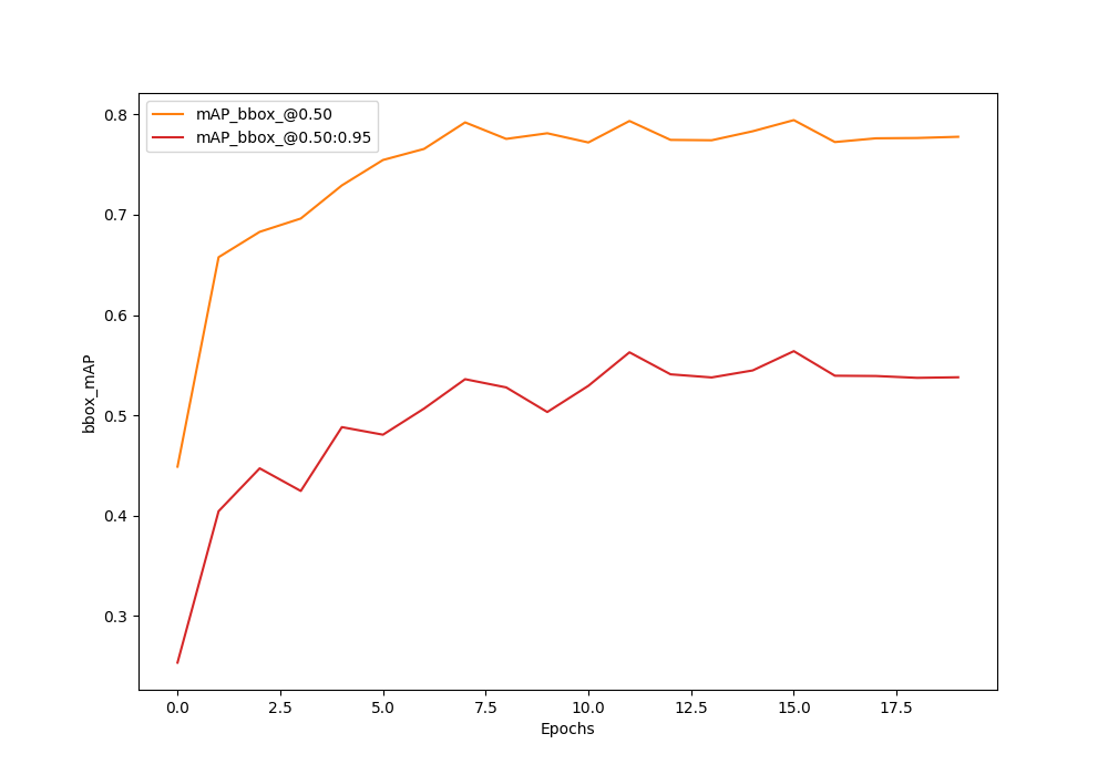
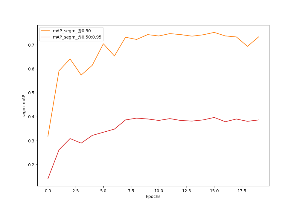
Figure 8. Bounding box mAP after training the Mask RCNN model on the lane detection dataset.

Figure 9. Segmentation mAP after training the Mask RCNN model on the lane detection dataset.

As we can see, the mAP was increasing for both till epoch 15. Most probably, if we apply another learning rate scheduler step after epoch 20, we can train even longer. For now, we will move forward with the best model weights from epoch 16.

Inference on Images using the Trained Mask RCNN Model

We have the Mask RCNN checkpoints trained on the lane detection and segmentation dataset. We can use the inference_image.py script to run inference on the validation images from the dataset and see how it performs.

Note: The inference scripts (image and video) by default load the Faster RCNN ResNet50 FPN V2 model as that’s what we used during training.

Executing the following command will carry out inference on the validation images.

python inference_image.py --weights outputs/training/road_line/model_15.pth --threshold 0.8 --input input/road_lane_instance_segmentation/val2017/ --show

Here are the command line arguments that we use:

--weights: Path to the weights file. We are using the weights from epoch 16 here.
--threshold: We are using a confidence threshold of 0.8.
--input: Path to the input directory containing the images.
--show: This is a boolean argument indicating that we want to visualize all the images on the screen as the inference is going on.

All the results are stored in outputs/inference directory.

Here are some of the results.

Figure 10. Inference results with bounding boxes and masks after training on the lane detection dataset.

The results are pretty good. It is detecting almost all the lines correctly even during the nighttime.

To get an even clearer picture, we can disable the bounding boxes using the --no-boxes argument.

python inference_image.py --weights outputs/training/road_line/model_15.pth --threshold 0.8 --input input/road_lane_instance_segmentation/val2017/ --show --no-boxes

This will plot just the segmentation maps. Here are some of the results.

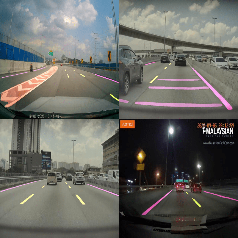
Figure 11. Inference results without bounding boxes after training on the lane detection dataset.

We can see that the model is performing pretty well on the validation images.

But these images are from the same distribution as the training images. Let’s make it more challenging and run inference on some unseen videos.

Lane Detection Inference on Videos using the Trained Mask RCNN Model

We will carry out inference on two videos. For this, we will take the help of the inference_video.py script.

Let’s start with a video on which the model performs relatively well.

python inference_video.py --weights outputs/training/road_line/model_15.pth --show --threshold 0.9 --input input/inference_data/video_3.mp4 --no-boxes

Almost all the command line arguments remain the same apart from the input file which is now a video. Also, we are using a score threshold of 0.9.

Clip 1. Real-time inference for lane detection using the Mask RCNN model.

The results look really good. The model is able to segment the solid lines and dotted lines in almost all the frames. It is able to run at an average of 17 FPS on the RTX 3080 GPU.

Next, let’s run inference on a video where the model performs relatively worse. We are just changing the video path here.

python inference_video.py --weights outputs/training/road_line/model_15.pth --show --threshold 0.9 --input input/inference_data/video_1.mp4 --no-boxes

Clip 2. Real-time inference for lane detection using Mask RCNN. Here the model does not perform very well.

Firstly, the model is not able to segment all the dotted lanes on the left. Secondly, it is detecting the dotted lanes on the right as solid lanes in some of the frames.

This shows the issues with out-of-distribution inference. We can improve the performance on such real-world videos by including such data in the training set. This will help us train a more robust lane detection Mask RCNN model.

Summary and Conclusion

In this article, we trained a Mask RCNN model for lane detection and segmentation. We approached the problem with an instance segmentation solution. The results were fairly good. However, we saw some limitations and discussed how we can improve upon them. I hope that this article was worth your time.

If you have any doubts, thoughts, or suggestions, please leave them in the comment section. I will surely address them.

You can contact me using the Contact section. You can also find me on LinkedIn, and Twitter.

References

Liked it? Take a second to support Sovit Ranjan Rath on Patreon!

Lane Detection using Mask RCNN – An Instance Segmentation Approach