Traffic Sign Detection using DETR

In this article, we will create a small proof of concept for traffic sign detection. We will use the DETR object detection model in particular for traffic sign detection. We will use a very small dataset. Also, we will entirely focus on the practical steps that we take to get the best results.

Traffic sign detection is an important problem in both autonomous driving and traffic surveillance. Object detection methods help in automating the process to a good extent. But solving it on a large scale requires a huge amount of data, engineering, and proper pipelines. In this article, however, we will train a few DETR object detection models on a small-scale traffic sign detection dataset. This will help us uncover how easy or difficult the process is.

We will cover the following points in this article:

• We will start with a discussion of the Tiny LISA Traffic Sign detection dataset.
• Then we will discuss the DETR (Detection Transformer) models that we will train on the traffic sign detection dataset.
• While discussing the technical part, we will particularly focus on dataset preparation and data augmentation techniques.
• After training, we will analyze the results of each training experiment.
• Next, we will run inference on a video to check the real-time performance of the trained DETR model.
• Finally, we will discuss a few points that will improve the project further.

The Tiny LISA Traffic Sign Detection Dataset

We will use the Tiny LISA Traffic Sign Detection Dataset that is available on Kaggle. This is a subset of the larger LISA traffic sign detection dataset.

There are only 900 images in this version of the dataset with a CSV annotation file. As the training codebase that we will use requires the annotations in XML format, we will do some preprocessing in the next section.

The dataset contains 9 object classes in this tiny version of the dataset.

• keepRight
• merge
• pedestrianCrossing
• signalAhead
• speedLimit25
• speedLimit35
• stop
• yield
• yeildAhead

For now, you may go ahead and download the dataset. After extracting it, you will find the following structure of the original dataset:

db_lisa_tiny/
├── annotations.csv
├── sample_001.png
├── sample_002.png
├── sample_003.png
├── sample_004.png
├── sample_005.png
├── sample_006.png
...
├── sample_899.png
└── sample_900.png

There are 900 images and one annotation file in the CSV format.

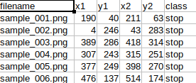
As we can see, there are six columns. The first is the filename of the image in the directory. The next four are the bounding box coordinates in <xmin, ymin, xmax, ymax> format. And the final one is the class name. However, there is one problematic thing in the dataset. We can see that there is only one annotation per image. This can lead to performance issues while training where the model only learns to detect one object in an image.

Analyzing the Tiny LISA Traffic Sign Detection Images with Annotations

Let’s take a look at a few images and annotations from the dataset.

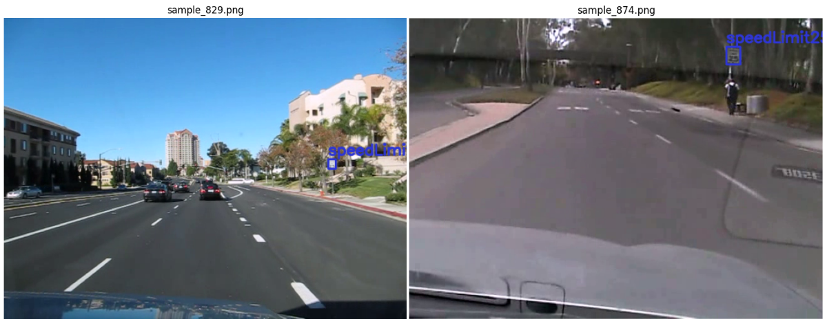
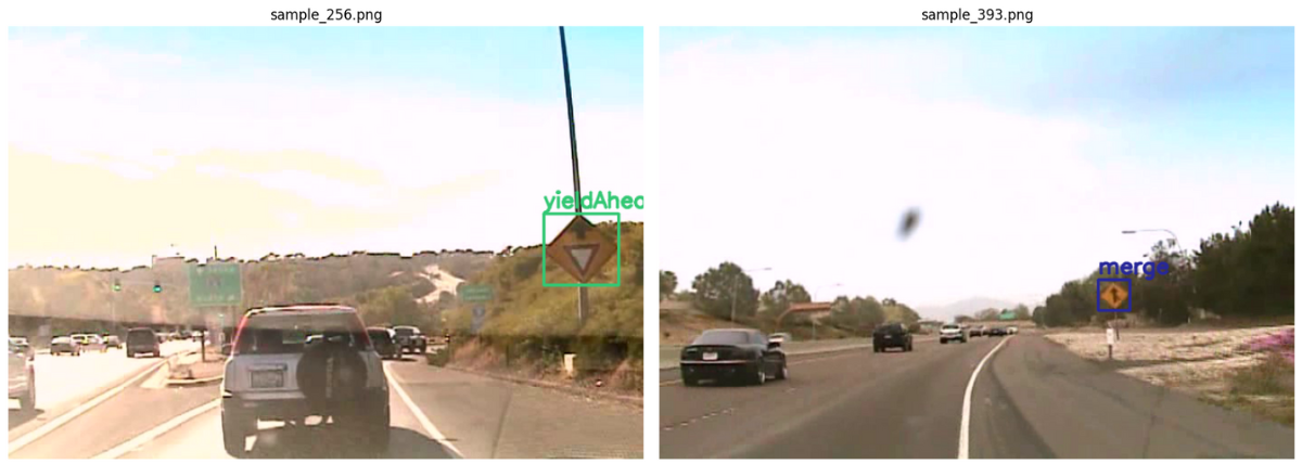
The images look quite challenging. As all the videos were captured from a dashcam, the frames are blurry, pixelated, and have different lighting depending on the time of the day. It will be a good challenge for the DETR model.

The Project Directory Structure

Now, let’s take a look at the entire project directory structure.

├── input
│   ├── db_lisa_tiny
│   ├── inference_data
│   ├── train_annots
│   ├── train_images
│   ├── valid_annots
│   ├── valid_images
│   ├── train.csv
│   └── valid.csv
├── notebooks
│   └── visualizations.ipynb
├── vision_transformers
│   ├── data
│   ├── examples
│   ├── example_test_data
│   ├── readme_images
│   ├── runs
│   ├── tools
│   ├── vision_transformers
│   ├── LICENSE
│   ├── requirements.txt
│   └── setup.py
├── csv_to_xml.py
└── split_data.py

• The input directory contains all the data that we need. The db_lisa_tiny is the original dataset directory that we saw above with 900 images and one CSV file. However, it does not contain any splits. So, after creating the splits and the XML annotation files, we will get train_images, train_annots, valid_images, and valid_annots directories. Before we create these directories, we will also create the train.csv and valid.csv files.
• The notebooks directory contains a Jupyter Notebook that we can use for visualizing the images and annotations.
• Then we have the vision_transformers directory. This is a GitHub repository that we will later clone. This contains a lot of vision transformer models for classification and detection. I have been maintaining this project for a few months now and will expand it in the future.
• Directly inside the parent project directory, we have the csv_to_xml.py and split_data.py Python files. The former converts the CSV data to XML format and the latter creates the training and validation CSV files along with copying the split images into their new directories. We will use these later to obtain the complete dataset.

The trained weights and the data conversion files will be available via the download section of this article. If you wish to just run inference, please download the trained zip file which contains the trained weights. If you plan on training the model as well, please download the dataset and we will create the additional files and folders in the following sections.

Download Code

The Vision Transformers Repository

Please go ahead and download the content for this article. After extracting it, enter the directory and clone the Vision Transformers repository.

git clone https://github.com/sovit-123/vision_transformers.git

After cloning the repository, make it the current directory and install the library.

cd vision_transformers

pip install .

The above will install the repository as a library and also install PyTorch as a dependency.

In case you face PyTorch and CUDA issues, please install PyTorch 2.0.1 (the latest at the time of writing this) using the following command.

conda install pytorch torchvision torchaudio pytorch-cuda=11.7 -c pytorch -c nvidia

Installing Dependencies

Next, we need to install a few mandatory libraries. These are torchinfo and pycocotools. The requirements file inside the vision_transformers directory will handle it.

pip install -r requirements.txt

The above are the most important installation steps. In case you are missing any other libraries along the way, please install them.

Note: If you plan on running inference only, after downloading and extracting the content for this post, please copy the content of trained_weights directory into vision_transformers/runs/training directory. You may need to create runs/training directory as it only gets created after the first training experiment.

Small Scale Traffic Sign Detection using DETR

From here on, we will start the coding part.

The first thing that we need to do is create the training and validation CSV files, the data splits, and the XML files.

Preparing the Dataset

Note: The commands in this section (dataset preparation) should be executed within the parent project directory and not within the vision_transformers directory.

The very first step is creating the train_images & valid_images directories, and train.csv & and valid.csv files in the input directory.

For this, we need to execute the split_data.py script.

python split_data.py

After executing the command, please take a look in the input directory to ensure the new CSV files and directories are present.

The next step is creating the XML files. For this, we need to execute the csv_to_xml.py script twice. Once for the training data and once for the validation data.

python csv_to_xml.py --input input/train.csv --output input/train_annots

python csv_to_xml.py --input input/valid.csv --output input/valid_annots

In the above commands, we use the following command line arguments:

• --input: Path to the CSV file.
• --output: Path to the directory where we want to store the XML files.

After this, we have all the files and folders in the input directory as we observed in the directory tree structure. We can now move to the deep learning part of the project.

Preparing the Dataset YAML File

The YAML file inside vision_transformers/data directory contains all the information related to the dataset. This includes the paths to the image and label directories, the class names, and the number of classes.

For training the DETR model on the traffic sign detection dataset, we have the lisa_traffic.yaml file. Here are its contents:

# Images and labels direcotry should be relative to train.py
TRAIN_DIR_IMAGES: '../input/train_images'
TRAIN_DIR_LABELS: '../input/train_annots'
VALID_DIR_IMAGES: '../input/valid_images'
VALID_DIR_LABELS: '../input/valid_annots'

# Class names.
CLASSES: [
    '__background__',
    'keepRight',
    'merge',
    'pedestrianCrossing',
    'signalAhead',
    'speedLimit25',
    'speedLimit35',
    'stop',
    'yield',
    'yieldAhead'
]

# Number of classes (object classes + 1 for background).
NC: 10

# Whether to save the predictions of the validation set while training.
SAVE_VALID_PREDICTION_IMAGES: True

As we will execute the training script within the vision_transformers directory, all the paths to relative to that.

After the paths, we have the CLASSES attribute which includes all the object classes along with the __background__ class. The total number of classes, NC, is the total number of classes including the background class.

You will find this file within the downloaded zip file as well. You just need to copy it into the vision_transformers/data directory.

Let’s get into the training part now.

Training the DETR ResNet50 with Augmentation

We will start with training the DETR ResNet50 model which is the smallest among the four models available. We will train it with a lot of augmentations to avoid overfitting.

Most of the heavy lifting for dataset preparation is done by the datasets.py file inside vision_transformers/tool/utils directory.

We will pass a command line argument to augment the images while training. The script uses the following augmentations:

• Any one of Blur, MotionBlur, or MedianBlur
• ToGray
• RandomBrightnessContrast
• ColorJitter
• RandomGamma

Let’s take a look at a few images to observe how they look after applying augmentations.

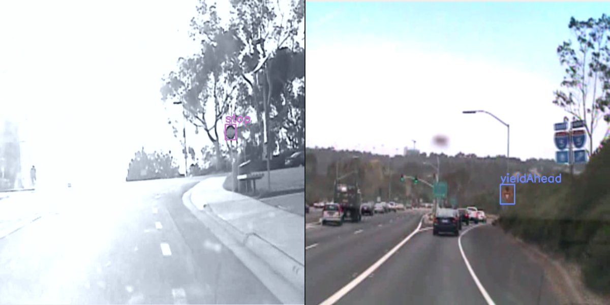
We can see that the augmentations add quite a lot of variability to the images. This will surely help in preventing overfitting.

Now, let’s execute the training command within the vision_transformers library.

python tools/train_detector.py --data data/lisa_traffic.yaml --epochs 75 --name detr_resnet50_75e --use-train-aug

The following are all the command line arguments that we use:

• --data: The path to the dataset YAML file.
• --epochs: The number of epochs to train for.
• --name: This is the directory name where all the results will be saved. For this training, it will be runs/training/detr_resnet50_75e
• --use-train-aug: This is a boolean argument indicating to use the training augmentations.

By default, the model is DETR ResNet50. So, we do not need to pass any model name here.

Analyzing the DETR ResNet50 Training Results

The following block shows the validation results from the best training epoch from the terminal. We track the mAP metric for object detection.

Test:  [ 0/23]  eta: 0:00:05  class_error: 0.00  loss: 0.4392 (0.4392)  loss_ce: 0.0236 (0.0236)  loss_bbox: 0.0504 (0.0504)  loss_giou: 0.3651 (0.3651)  loss_ce_unscaled: 0.0236 (0.0236)  class_error_unscaled: 0.0000 (0.0000)  loss_bbox_unscaled: 0.0101 (0.0101)  loss_giou_unscaled: 0.1825 (0.1825)  cardinality_error_unscaled: 0.0000 (0.0000)  time: 0.2340  data: 0.1748  max mem: 2204
Test:  [22/23]  eta: 0:00:00  class_error: 50.00  loss: 0.4169 (0.4326)  loss_ce: 0.0266 (0.0480)  loss_bbox: 0.0479 (0.0546)  loss_giou: 0.2933 (0.3300)  loss_ce_unscaled: 0.0266 (0.0480)  class_error_unscaled: 0.0000 (11.9565)  loss_bbox_unscaled: 0.0096 (0.0109)  loss_giou_unscaled: 0.1466 (0.1650)  cardinality_error_unscaled: 0.5000 (0.4130)  time: 0.0579  data: 0.0057  max mem: 2204
Test: Total time: 0:00:01 (0.0677 s / it)
Averaged stats: class_error: 50.00  loss: 0.4169 (0.4326)  loss_ce: 0.0266 (0.0480)  loss_bbox: 0.0479 (0.0546)  loss_giou: 0.2933 (0.3300)  loss_ce_unscaled: 0.0266 (0.0480)  class_error_unscaled: 0.0000 (11.9565)  loss_bbox_unscaled: 0.0096 (0.0109)  loss_giou_unscaled: 0.1466 (0.1650)  cardinality_error_unscaled: 0.5000 (0.4130)
Accumulating evaluation results...
DONE (t=0.07s).
IoU metric: bbox
 Average Precision  (AP) @[ IoU=0.50:0.95 | area=   all | maxDets=100 ] = 0.547
 Average Precision  (AP) @[ IoU=0.50      | area=   all | maxDets=100 ] = 0.815
 Average Precision  (AP) @[ IoU=0.75      | area=   all | maxDets=100 ] = 0.633
 Average Precision  (AP) @[ IoU=0.50:0.95 | area= small | maxDets=100 ] = 0.443
 Average Precision  (AP) @[ IoU=0.50:0.95 | area=medium | maxDets=100 ] = 0.565
 Average Precision  (AP) @[ IoU=0.50:0.95 | area= large | maxDets=100 ] = 0.714
 Average Recall     (AR) @[ IoU=0.50:0.95 | area=   all | maxDets=  1 ] = 0.643
 Average Recall     (AR) @[ IoU=0.50:0.95 | area=   all | maxDets= 10 ] = 0.716
 Average Recall     (AR) @[ IoU=0.50:0.95 | area=   all | maxDets=100 ] = 0.725
 Average Recall     (AR) @[ IoU=0.50:0.95 | area= small | maxDets=100 ] = 0.733
 Average Recall     (AR) @[ IoU=0.50:0.95 | area=medium | maxDets=100 ] = 0.892
 Average Recall     (AR) @[ IoU=0.50:0.95 | area= large | maxDets=100 ] = 0.716

BEST VALIDATION mAP: 0.5465645512672217

SAVING BEST MODEL FOR EPOCH: 71

The best model was saved after epoch number 72 (epoch index starts from 0). We have the best validation mAP of 54.7% using the DETR ResNet50 model.

Let’s take a look at the mAP graph.

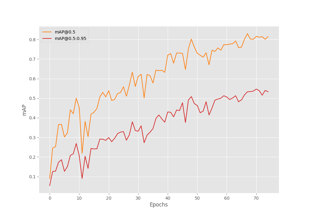
It looks like we could have trained for a few more epochs.

Training the DETR ResNet50 DC5 with Augmentation on the Traffic Sign Dataset

We will train another model here. It is the DETR ResNet50 DC5 model which is slightly better compared to the previous model. Basically, it uses dilated convolution so the features maps are double the size compared to the DETR ResNet50 model.

We just need one additional command line argument in this case.

python tools/train_detector.py --model detr_resnet50_dc5 --data data/lisa_traffic.yaml --epochs 75 --name detr_resnet50_dc5_75e --use-train-aug

This time we are passing a --model argument whose value is detr_resnet50_dc5. Also, the result directory --name is different.

Analyzing the DETR ResNet50 DC5 Training Results

The DETR ResNet50 DC5 model reaches the best mAP on epoch number 62.

Test:  [ 0/23]  eta: 0:00:06  class_error: 0.00  loss: 0.4462 (0.4462)  loss_ce: 0.0096 (0.0096)  loss_bbox: 0.0479 (0.0479)  loss_giou: 0.3887 (0.3887)  loss_ce_unscaled: 0.0096 (0.0096)  class_error_unscaled: 0.0000 (0.0000)  loss_bbox_unscaled: 0.0096 (0.0096)  loss_giou_unscaled: 0.1943 (0.1943)  cardinality_error_unscaled: 0.2500 (0.2500)  time: 0.2933  data: 0.1880  max mem: 7368
Test:  [22/23]  eta: 0:00:00  class_error: 0.00  loss: 0.3595 (0.3595)  loss_ce: 0.0090 (0.0200)  loss_bbox: 0.0370 (0.0427)  loss_giou: 0.2867 (0.2968)  loss_ce_unscaled: 0.0090 (0.0200)  class_error_unscaled: 0.0000 (5.4348)  loss_bbox_unscaled: 0.0074 (0.0085)  loss_giou_unscaled: 0.1434 (0.1484)  cardinality_error_unscaled: 0.2500 (0.3913)  time: 0.1007  data: 0.0061  max mem: 7368
Test: Total time: 0:00:02 (0.1111 s / it)
Averaged stats: class_error: 0.00  loss: 0.3595 (0.3595)  loss_ce: 0.0090 (0.0200)  loss_bbox: 0.0370 (0.0427)  loss_giou: 0.2867 (0.2968)  loss_ce_unscaled: 0.0090 (0.0200)  class_error_unscaled: 0.0000 (5.4348)  loss_bbox_unscaled: 0.0074 (0.0085)  loss_giou_unscaled: 0.1434 (0.1484)  cardinality_error_unscaled: 0.2500 (0.3913)
Accumulating evaluation results...
DONE (t=0.08s).
IoU metric: bbox
 Average Precision  (AP) @[ IoU=0.50:0.95 | area=   all | maxDets=100 ] = 0.629
 Average Precision  (AP) @[ IoU=0.50      | area=   all | maxDets=100 ] = 0.881
 Average Precision  (AP) @[ IoU=0.75      | area=   all | maxDets=100 ] = 0.708
 Average Precision  (AP) @[ IoU=0.50:0.95 | area= small | maxDets=100 ] = 0.617
 Average Precision  (AP) @[ IoU=0.50:0.95 | area=medium | maxDets=100 ] = 0.711
 Average Precision  (AP) @[ IoU=0.50:0.95 | area= large | maxDets=100 ] = 0.761
 Average Recall     (AR) @[ IoU=0.50:0.95 | area=   all | maxDets=  1 ] = 0.700
 Average Recall     (AR) @[ IoU=0.50:0.95 | area=   all | maxDets= 10 ] = 0.760
 Average Recall     (AR) @[ IoU=0.50:0.95 | area=   all | maxDets=100 ] = 0.768
 Average Recall     (AR) @[ IoU=0.50:0.95 | area= small | maxDets=100 ] = 0.800
 Average Recall     (AR) @[ IoU=0.50:0.95 | area=medium | maxDets=100 ] = 0.875
 Average Recall     (AR) @[ IoU=0.50:0.95 | area= large | maxDets=100 ] = 0.762

BEST VALIDATION mAP: 0.6292527183321788

SAVING BEST MODEL FOR EPOCH: 61

This time, we have a much higher mAP of 62.9% on the traffic sign detection dataset.

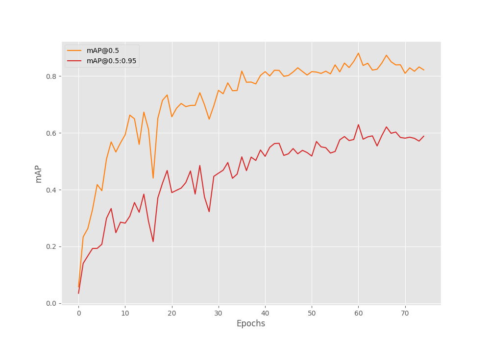
It is clearly visible that the model has already started overfitting. So, training for any longer would not be beneficial.

As the DETR ResNet50 DC5 model has a better object detection metric, we will use this model for inference next.

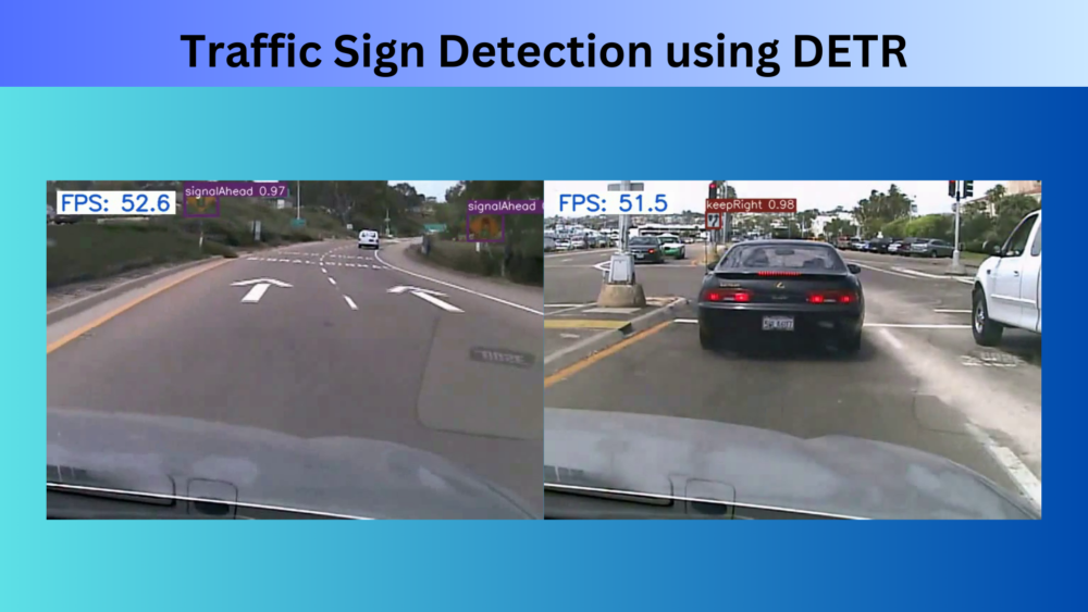
Traffic Sign Detection Video Inference

As we have the best weights for the DETR ResNet50 DC5 model, we will use that for video inference.

The video that we will use has been generated from the original full set of LISA Traffic Sign Detection data. The frames were combined at 15 FPS to create a small video. You will find that within the downloadable zip file that comes with this article.

We will use inference_video_detect.py script inside the tools directory to run the inference. We will execute the following command within the vision_transformers directory.

python tools/inference_video_detect.py --input ../input/inference_data/video_1.mp4 --weights runs/training/detr_resnet50_dc5_75e/best_model.pth --show --imgsz 640

The following are the command line arguments that we use:

• --input: The path to the input video.
• --weights: Path to the best trained weights.
• --show: This is a boolean argument indicating that we want to visualize the inference on screen.
• --imgsz: This takes in an integer and the images will be resized to the square size of whatever value we pass. So, in this case, the images will be resized to 640×640 resolution.

The results will be saved in runs/inference directory.

Note: There are some repeated frames in the original dataset.

As we can see, the model is able to detect most of the objects correctly. However, there are a few wrong detections. For example, wherever there are signs of a speed limit other than 25 or 35, the model is detecting them as either speedLimit25 or speedLimit35. This is not entirely the model’s fault as it never got to see those objects and annotations during training.

Other than that, the model is able to detect multiple objects in a scene even though no multiple annotations were present in a single image.

Further Improvements

To make the training process even more robust, we can train it on the entire LISA Traffic Sign Detection dataset which contains more than 6000 images and 49 classes.

We will try to tackle this in a future post.

Summary and Conclusion

In this article, we trained DETR object detection models to detect traffic signs. We trained the models on the Tiny LISA Traffic Sign Detection dataset and compared their performances. After that, we also ran video inference and saw how the best model is performing. Finally, we discussed some improvement points. I hope that this article was worth your time.

If you have any doubts, thoughts, or suggestions, please leave them in the comment section. I will surely address them.

You can contact me using the Contact section. You can also find me on LinkedIn, and Twitter.