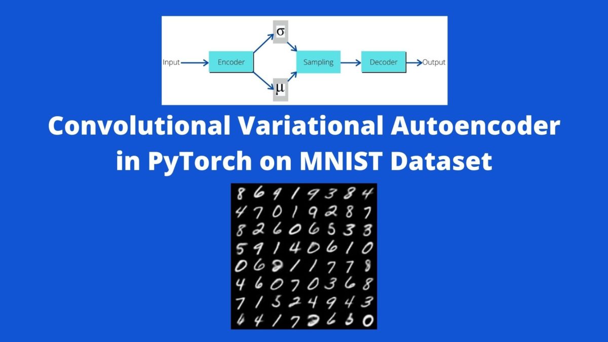
In this tutorial, you will get to learn to implement the convolutional variational autoencoder using PyTorch. In particular, you will learn how to use a convolutional variational autoencoder in PyTorch to generate the MNIST digit images.
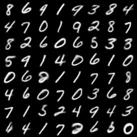
Figure 1. Result of MNIST digit reconstruction using convolutional variational autoencoder neural network.
Figure 1 shows what kind of results the convolutional variational autoencoder neural network will produce after we train it. You can hope to get similar results. Let’s move ahead then. And the best part is how variational autoencoders seem to transition from one digit image to another as they begin to learn the data more. We will see this in full action in this tutorial.
Note: We will skip most of the theoretical concepts in this tutorial. Instead, we will focus on how to build a proper convolutional variational autoencoder neural network model. I have covered the theoretical concepts in my previous articles. I will be linking some specific one of those a bit further on.
A Bit of Background
A few days ago, I got an email from one of my readers. He is trying to generate MNIST digit images using variational autoencoders. But he was facing some issues. He said that the neural network’s loss was pretty low. Still, the network was not able to generate any proper images even after 50 epochs.
That was a bit weird as the autoencoder model should have been able to generate some plausible images after training for so many epochs. There can be either of the two major reasons for this:
Either the stacking of the convolutional variational autoencoder layers is wrong.
Or, the selection of mean and log variance from the latent space encoding is done in the wrong way. This will result in a wrong reparameterization trick and will lead to wrong results.
Again, it is a very common issue to run into this when learning and trying to implement variational autoencoders in deep learning. Variational autoencoders can be sometimes hard to understand and I ran into these issues myself. For this reason, I have also written several tutorials on autoencoders. This helped me in understanding everything in a much better way.
If you are very new to autoencoders in deep learning, then I would suggest that you read these two articles first:
Autoencoders in Deep Learning: Get to know the basics of autoencoder neural networks in deep learning from this one.
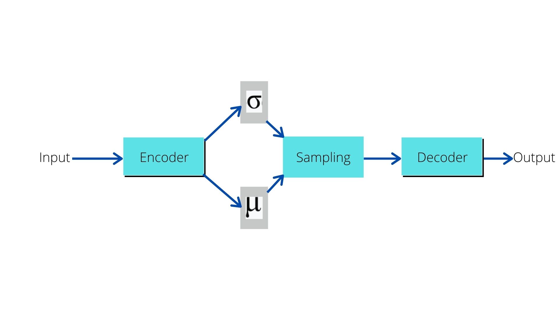
Figure 2. The architecture of a variational autoencoder neural network. To get more details about the working of variational autoencoder, you can click here.
Difference Between Standard Autoencoders and Variational Autoencoders
We will not go into the very details of this topic. Just to set a background:
Standard autoencoders: They produce data/images from the latent vector. But they try to replicate or copy the image data while doing so.
Variational autoencoder: They are good at generating new images from the latent vector. Although they generate new data/images, still, those are very similar to the data they are trained on.
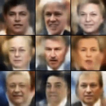
We can have a lot of fun with variational autoencoders if we can get the architecture and reparameterization trick right. For example, take a look at the following image.
Figure 3. Fictional celebrity faces that are created by a convolutional variational autoencoder neural network (Source).
Figure 3 shows the images of fictional celebrities that are generated by a variational autoencoder. It would be real fun to take up such a project. But we will stick to the basic of building architecture of the convolutional variational autoencoder in this tutorial. Maybe we will tackle this and working with RGB images in a future article.
Again, you can get all the basics of autoencoders and variational autoencoders from the links that I have provided in the previous section. Do take a look at them if you are new to autoencoder neural networks in deep learning.
Libraries and Project Directory Structure
We will use PyTorch in this tutorial. For this project, I have used the PyTorch version 1.6. Although any older or newer versions should work just fine as well. We will be using the most common modules for building the autoencoder neural network architecture.
As for the project directory structure, we will use the following.
The input folder will contain the MNIST dataset that we will download from torchvision.datasets.
Inside the outputs folder, all the generated images, and loss plots will be stored while training and validation are going on.
And src contains our four python scripts. We will get into the details of these while writing the code for each of them.
Now, we are all ready with our setup, let’s start the coding part.
Convolutional Variational Autoencoder using PyTorch
We will write the code inside each of the Python scripts in separate and respective sections. We will start with writing some utility code which will help us along the way.
Writing the Utility Code
Here, we will write the code inside the utils.py script. This will contain some helper as well as some reusable code that will help us during the training of the autoencoder neural network model. Be sure to create all the .py files inside the src folder.
We will write the following code inside utils.py script.
import imageio
import numpy as np
import torchvision.transforms as transforms
import matplotlib.pyplot as plt

from torchvision.utils import save_image

to_pil_image = transforms.ToPILImage()

def image_to_vid(images):
    imgs = [np.array(to_pil_image(img)) for img in images]
    imageio.mimsave('../outputs/generated_images.gif', imgs)


def save_reconstructed_images(recon_images, epoch):
    save_image(recon_images.cpu(), f"../outputs/output{epoch}.jpg")

def save_loss_plot(train_loss, valid_loss):
    # loss plots
    plt.figure(figsize=(10, 7))
    plt.plot(train_loss, color='orange', label='train loss')
    plt.plot(valid_loss, color='red', label='validataion loss')
    plt.xlabel('Epochs')
    plt.ylabel('Loss')
    plt.legend()
    plt.savefig('../outputs/loss.jpg')
    plt.show()
Let’s go over the important parts of the above code.
First of all, we are importing the imageio library. This will help us save all the image reconstruction by the autoencoder neural network model from each epoch as a .gif file. To do that, we will need to convert all the variational autoencoder reconstructions to PIL image format. We are defining a transform for that at line 8.
At line 10, we define the image_to_vid() function which accepts an images parameter. This list contains all the reconstructed images. We are converting those to NumPy array format and then saving them as a .gif file.
We will also be saving all the static images that are reconstructed by the variational autoencoder neural network. The save_reconstructed_images() function does that. It accepts the reconstructed image and the epoch number and saves those images.
Finally, starting from line 18, we have the save_loss_plot() function which saves the training and validation graphical loss plots.
The above are the utility codes that we will be using while training and validating.
Define the Training, Validation, and Loss Functions
In this section, we will define three functions. One is the loss function for the variational convolutional autoencoder. The other two are the training and validation functions. All of this code will go into the engine.py script.
The Loss Function for the Variational Autoencoder Neural Network
If you have some experience with variational autoencoders in deep learning, then you may be knowing that the final loss function is a combination of the reconstruction loss and the KL Divergence.
For the reconstruction loss, we will use the Binary Cross-Entropy loss function. As for the KL Divergence, we will calculate it from the mean and log variance of the latent vector.
Again, if you are new to all this, then I highly recommend going through this article.
The following block of code imports and required modules and defines the final_loss() function.
from tqdm import tqdm

import torch

def final_loss(bce_loss, mu, logvar):
    """
    This function will add the reconstruction loss (BCELoss) and the
    KL-Divergence.
    KL-Divergence = 0.5 * sum(1 + log(sigma^2) - mu^2 - sigma^2)

    :param bce_loss: recontruction loss
    :param mu: the mean from the latent vector
    :param logvar: log variance from the latent vector
    """
    BCE = bce_loss
    KLD = -0.5 * torch.sum(1 + logvar - mu.pow(2) - logvar.exp())

    return BCE + KLD
The loss function accepts three input parameters, they are the reconstruction loss, the mean, and the log variance.
The reconstruction loss, bce_loss is the loss from the images reconstructed by the convolutional variational autoencoder neural network and the original data. We get the mean mu and the log variance log_var from the autoencoder’s latent space encoding.
We calculate the KL divergence (KLD) at line 16 and return the total loss at line 18.
You will find the details regarding the loss function and KL divergence in the article mentioned above.
The Training Function
The training function is going to be really simple yet important for the proper learning of the autoencoder neural neural network. Hopefully, the training function will make it clear how we are using the above loss function.
The following is the complete training function.
def train(model, dataloader, dataset, device, optimizer, criterion):
    model.train()
    running_loss = 0.0
    counter = 0
    for i, data in tqdm(enumerate(dataloader), total=int(len(dataset)/dataloader.batch_size)):
        counter += 1
        data = data[0]
        data = data.to(device)
        optimizer.zero_grad()
        reconstruction, mu, logvar = model(data)
        bce_loss = criterion(reconstruction, data)
        loss = final_loss(bce_loss, mu, logvar)
        loss.backward()
        running_loss += loss.item()
        optimizer.step()

    train_loss = running_loss / counter
    return train_loss
The train() function accepts six parameters. They are the autoencoder model, the training data loader, the training set, the computation device, optimizer, and the loss function (criterion).
We define a running_loss variable at line 21 to keep track of the batch-wise loss values while training. We also initialize a counter variable to keep track of the total number of training steps.
The training loop begins at line 23. Notice that we are capturing only the image data at line 25 as we do not need the labels to train our convolutional variational autoencoder.
At line 28, we pass the data through the model. This returns us the reconstruction, mu, and logvar.
Using the reconstructed image data, we calculate the BCE Loss at line 29.
Then we calculate the final loss value for the current batch at line 30. This we do by calling the final_loss() function and passing the loss, mu, and log_var as the arguments.
After that, all the general steps like backpropagating the loss and updating the optimizer parameters happen.
Finally, we return the training loss for the current epoch after calculating it at line 36.
I hope that the training function clears some of the doubt about the working of the loss function.
The Validation Function
The validation function will be a bit different from the training function. Apart from the fact that we do not backpropagate the loss and update the optimizer parameters, we also need the image reconstructions from the validation function. This we will save to the disk for later anaylis.
The following code block define the validation function.
def validate(model, dataloader, dataset, device, criterion):
    model.eval()
    running_loss = 0.0
    counter = 0
    with torch.no_grad():
        for i, data in tqdm(enumerate(dataloader), total=int(len(dataset)/dataloader.batch_size)):
            counter += 1
            data= data[0]
            data = data.to(device)
            reconstruction, mu, logvar = model(data)
            bce_loss = criterion(reconstruction, data)
            loss = final_loss(bce_loss, mu, logvar)
            running_loss += loss.item()

            # save the last batch input and output of every epoch
            if i == int(len(dataset)/dataloader.batch_size) - 1:
                recon_images = reconstruction

    val_loss = running_loss / counter
    return val_loss, recon_images
The validate() function accepts the model, the validation data loader, the validation dataset, the computation device, and the loss function as parameters.
The validation happens within the with torch.no_grad() block as we do not need to calculate the gradients here.
The important line here is line 52. If we are at the last batch of every epoch, then we save the reconstructed images as recon_images. This we return with the final validation loss at line 56.
So, basically, we are capturing one reconstruction image data from each epoch and we will be saving that to the disk. We will also use these reconstructed images to create a final .gif file. This will allow us to see the convolutional variational autoencoder in full action and how it reconstructs the images as it begins to learn more about the data.
This is all we need for the engine.py script. Now, we will move on to prepare our convolutional variational autoencoder model in PyTorch.
Prepare the Convolutional Variational Autoencoder Model
Now, we will move on to prepare the convolutional variational autoencoder model. We will try our best and focus on the most important parts and try to understand them as well as possible.
All of this code will go into the model.py Python script.
Let’s start with the required imports and the initializing some variables.
import torch
import torch.nn as nn
import torch.nn.functional as F

kernel_size = 4 # (4, 4) kernel
init_channels = 8 # initial number of filters
image_channels = 1 # MNIST images are grayscale
latent_dim = 16 # latent dimension for sampling
There are some values which will not change much or at all.
The kernel_size is going to be 4×4 for all of the convolutional and transposed convolutional layers of the autoencoder model.
The init_channels are the first convolutional layer’s output channels. We will double this value with each passing convolutional layer. Similarly, we will half the value for each of the transposed convolutional layers.
We have image_channels = 1 as we are using MNIST images which are grayscale images.
Finally, the latent_dim defines the sampling feature value for the fully connected layers.
All of the values will begin to make more sense when we actually start to build our model using them. So, let’s move ahead with that.
Defining the Convolutional Variational Autoencoder Class
We will define our convolutional variational autoencoder model class here. I will be providing the code for the whole model within a single code block. This is to maintain the continuity and to avoid any indentation confusions as well. After the code, we will get into the details of the model’s architecture.
# define a Conv VAE
class ConvVAE(nn.Module):
    def __init__(self):
        super(ConvVAE, self).__init__()

        # encoder
        self.enc1 = nn.Conv2d(
            in_channels=image_channels, out_channels=init_channels, kernel_size=kernel_size,
            stride=2, padding=1
        )
        self.enc2 = nn.Conv2d(
            in_channels=init_channels, out_channels=init_channels*2, kernel_size=kernel_size,
            stride=2, padding=1
        )
        self.enc3 = nn.Conv2d(
            in_channels=init_channels*2, out_channels=init_channels*4, kernel_size=kernel_size,
            stride=2, padding=1
        )
        self.enc4 = nn.Conv2d(
            in_channels=init_channels*4, out_channels=64, kernel_size=kernel_size,
            stride=2, padding=0
        )

        # fully connected layers for learning representations
        self.fc1 = nn.Linear(64, 128)
        self.fc_mu = nn.Linear(128, latent_dim)
        self.fc_log_var = nn.Linear(128, latent_dim)
        self.fc2 = nn.Linear(latent_dim, 64)

        # decoder
        self.dec1 = nn.ConvTranspose2d(
            in_channels=64, out_channels=init_channels*8, kernel_size=kernel_size,
            stride=1, padding=0
        )
        self.dec2 = nn.ConvTranspose2d(
            in_channels=init_channels*8, out_channels=init_channels*4, kernel_size=kernel_size,
            stride=2, padding=1
        )
        self.dec3 = nn.ConvTranspose2d(
            in_channels=init_channels*4, out_channels=init_channels*2, kernel_size=kernel_size,
            stride=2, padding=1
        )
        self.dec4 = nn.ConvTranspose2d(
            in_channels=init_channels*2, out_channels=image_channels, kernel_size=kernel_size,
            stride=2, padding=1
        )

    def reparameterize(self, mu, log_var):
        """
        :param mu: mean from the encoder's latent space
        :param log_var: log variance from the encoder's latent space
        """
        std = torch.exp(0.5*log_var) # standard deviation
        eps = torch.randn_like(std) # `randn_like` as we need the same size
        sample = mu + (eps * std) # sampling
        return sample

    def forward(self, x):
        # encoding
        x = F.relu(self.enc1(x))
        x = F.relu(self.enc2(x))
        x = F.relu(self.enc3(x))
        x = F.relu(self.enc4(x))

        batch, _, _, _ = x.shape
        x = F.adaptive_avg_pool2d(x, 1).reshape(batch, -1)
        hidden = self.fc1(x)

        # get `mu` and `log_var`
        mu = self.fc_mu(hidden)
        log_var = self.fc_log_var(hidden)

        # get the latent vector through reparameterization
        z = self.reparameterize(mu, log_var)
        z = self.fc2(z)

        z = z.view(-1, 64, 1, 1)

        # decoding
        x = F.relu(self.dec1(z))
        x = F.relu(self.dec2(x))
        x = F.relu(self.dec3(x))
        reconstruction = torch.sigmoid(self.dec4(x))
        return reconstruction, mu, log_var
We Will Start with the Encoder Explanation
Starting from line 15, we define the variational autoencoder’s encoder part. This only consists of 2D convolutional layers.
The number of input and output channels are 1 and 8 respectively. Remember that we have initialized init_channels with 8 in the previous code block.
We have a total of four convolutional layers making up the encoder part of the network. And with each passing convolutional layer, we are doubling the number of output channels.
The kernel_size is 4×4 for all the layers. We have a stride of 2 for each layer as well. Along with that padding is 1 for the first three convolutional layers and 0 for the last one.
Having a large kernel size and stride of 2 will ensure that each time we are capturing a lot of spatial information and we are doing that repeatedly as well.
With the convolutional layers, our autoencoder neural network will be able to learn all the spatial information of the images.
Moving On to the Fully Connected Layers
After the convolutional layers, we have the fully connected layers starting from line 33. We have a total of four fully connected dense layers.
self.fc1 at line 33 has 64 input features and 128 output features.
Then we have self.fc_mu and self.fc_log_var. Both of these have 128 input features and 16 output features defined by latent_dim. Now, these two fully connected layers are responsible for providing us the mean and log variance value from this bottleneck part. We will do the sampling using these features and in-turn this will lead to the reconstruction of the images. We will see that part shortly.
For the final fully connected layer, we have 16 input features and 64 output features.
You may have a question, why do we have a fully connected part between the encoder and decoder in a “convolutional variational autoencoder”?
Well, the convolutional encoder will help in learning all the spatial information about the image data. Then the fully connected dense features will help the model to learn all the interesting representations of the data. A dense bottleneck will give our model a good overall view of the whole data and thus may help in better image reconstruction finally.
The Decoder Part of the Neural Network
Starting from line 39, we have the decoder part of the neural network.
This is just the opposite of the encoder part of the network.
With each transposed convolutional layer, we half the number of output channels until we reach at self.dec4.
The kernel_size is 4×4 for all layers, stride is 2. We start with a padding of 0 and 1 for the rest of the three transposed convolutions.
We have defined all the layers that we need to build up our convolutional variational autoencoder. Further, we will move into some of the important functions that will execute while the data passes through our model.
The Reparameterization Trick
The reparameterize() function is the place where most of the magic happens. This can be said to be the most important part of a variational autoencoder neural network.
The reparameterize() function accepts the mean mu and log variance log_var as input parameters. Both of these come from the autoencoder’s latent space encoding.
First, we calculate the standard deviation std and then generate eps which is the same size as std. The sampling at line 63 happens by adding mu to the element-wise multiplication of std and eps. This is known as the reparameterization trick.
The forward() Function
The forward() function starts from line 66. It is going to be real simple.
First, the encoding of the data happens line 68 through 71. We apply ReLU activation to each of the encoding layer.
From line 73 till 75, we reshape the data and apply the first fully-connected layer.
Then we calculate mu and log_var at lines 78 and 79.
Using mu and log_var we get the sampling through reparameterization at line 82 and this we pass through the final fully connected layer.
We make the sample four dimensional at line 85 so that it be given as an input to the transposed convolutional layers.
In the decoding part (from line 88), we apply ReLU activation to the first three transposed convolutional layers. Then at line 91, the final decoder layer returns the reconstruction of the data by applying the Sigmoid activation.
Finally, we return reconstruction, mu, and log_var at line 92.
That was a lot of theory, but I hope that you were able to know the flow of data through the variational autoencoder model.
Training Our Convolutional Variational Autoencoder in PyTorch on MNIST Dataset
We are all set to write the training code for our small project. This part is going to be the easiest. And many of you must have done training steps similar to this before. The following are the steps:
We will initialize the model and load it onto the computation device.
Prepare the training and validation data loaders.
Train our convolutional variational autoencoder neural network on the MNIST dataset for 100 epochs.
Save the reconstructions and loss plots.
Analyze the results.
So, let’s begin. We start with importing all the required modules, including the ones that we have written as well.
import torch
import torch.optim as optim
import torch.nn as nn
import model
import torchvision.transforms as transforms
import torchvision
import matplotlib

from torch.utils.data import DataLoader
from torchvision.utils import make_grid
from engine import train, validate
from utils import save_reconstructed_images, image_to_vid, save_loss_plot

matplotlib.style.use('ggplot')
Along with all other, we are also importing our own model, and the required functions from engine, and utils.
Setting the Computation Device and Learning Parameters
The following block of code initializes the computation device and the learning parameters to be used while training.
device = torch.device('cuda' if torch.cuda.is_available() else 'cpu')

# initialize the model
model = model.ConvVAE().to(device)

# set the learning parameters
lr = 0.001
epochs = 100
batch_size = 64
optimizer = optim.Adam(model.parameters(), lr=lr)
criterion = nn.BCELoss(reduction='sum')

# a list to save all the reconstructed images in PyTorch grid format
grid_images = []
We are defining the computation device at line 15. A GPU is not strictly necessary for this project. But of course, it will result in faster training if you have one. Still, you can move ahead with the CPU as your computation device. We are initializing the deep learning model at line 18 and loading it onto the computation device.
For, the learning parameters:
We are using learning a learning rate of 0.001.
We will train for 100 epochs with a batch size of 64.
The optimizer is Adam optimizer.
And we we will be using BCELoss (Binary Cross-Entropy) as the reconstruction loss function.
We also have a list grid_images at line 28. After each training epoch, we will be appending the image reconstructions to this list. Then we will use it to generate our .gif file containing the reconstructed images from all the training epochs.
Prepare the Dataset
This part will contain the preparation of the MNIST dataset and defining the image transforms as well. We will not go into much detail here.
transform = transforms.Compose([
    transforms.Resize((32, 32)),
    transforms.ToTensor(),
])

# training set and train data loader
trainset = torchvision.datasets.MNIST(
    root='../input', train=True, download=True, transform=transform
)
trainloader = DataLoader(
    trainset, batch_size=batch_size, shuffle=True
)

# validation set and validation data loader
testset = torchvision.datasets.MNIST(
    root='../input', train=False, download=True, transform=transform
)
testloader = DataLoader(
    testset, batch_size=batch_size, shuffle=False
)
For the transforms, we are resizing the images to 32×32 size instead of the original 28×28. Then we are converting the images to PyTorch tensors.
Then, we are preparing the trainset, trainloader and testset, testloader for training and validation.
The Training Loop
As discussed before, we will be training our deep learning model for 100 epochs. The following is the training loop for training our deep learning variational autoencoder neural network on the MNIST dataset.
train_loss = []
valid_loss = []
for epoch in range(epochs):
    print(f"Epoch {epoch+1} of {epochs}")
    train_epoch_loss = train(
        model, trainloader, trainset, device, optimizer, criterion
    )
    valid_epoch_loss, recon_images = validate(
        model, testloader, testset, device, criterion
    )
    train_loss.append(train_epoch_loss)
    valid_loss.append(valid_epoch_loss)

    # save the reconstructed images from the validation loop
    save_reconstructed_images(recon_images, epoch+1)
    # convert the reconstructed images to PyTorch image grid format
    image_grid = make_grid(recon_images.detach().cpu())
    grid_images.append(image_grid)
    print(f"Train Loss: {train_epoch_loss:.4f}")
    print(f"Val Loss: {valid_epoch_loss:.4f}")
First, we have train_loss and valid_loss lists. We will store all the epoch-wise loss values in these two lists.
Starting from line 51 we have our training loop. We are passing the required arguments to the train() and validate() functions. We are appending the loss values from each epoch to train_loss and valid_loss at lines 59 and 60.
At line 63, we are saving the reconstructed images that our variational autoencoder neural network outputs.
Line 65 converts the reconstructed images to image grids by using the make_grid() function from PyTorch. Then we are just appending those grid images to the grid_images list.
Finally, we just need to save the grid images as .gif file and save the loss plot to the disk. The following block of code does that for us.
# save the reconstructions as a .gif file
image_to_vid(grid_images)

# save the loss plots to disk
save_loss_plot(train_loss, valid_loss)

print('TRAINING COMPLETE')
We are done with our coding part now. Its time to train our convolutional variational autoencoder neural network and see how it performs.
Executing train.py for Training Our Neural Network Model
Open up your command line/terminal and cd into the src folder of the project directory. From there, execute the following command.
python train.py
You should see output similar to the following.
Epoch 1 of 100
938it [00:13, 69.47it/s]
157it [00:01, 118.45it/s]
Train Loss: 15893.2751
Val Loss: 12067.1350
Epoch 2 of 100
...
Epoch 100 of 100
938it [00:13, 70.40it/s]
157it [00:01, 117.54it/s]
Train Loss: 9475.2831
Val Loss: 9524.0136

TRAINING COMPLETE
Analyzing the Loss Plot
Now, as our training is complete, let’s move on to take a look at our loss plot that is saved to the disk.
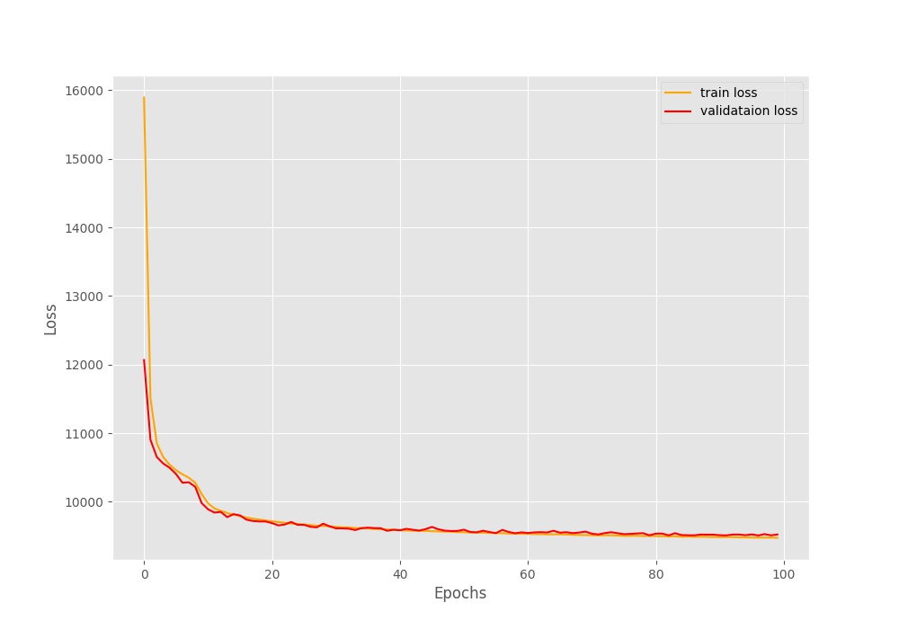
Figure 4. The loss plot after training the convolutional variational autoencoder neural network in PyTorch for 100 epochs. The loss seems to be decreasing till the end of training.
Here, the loss seems to start at a pretty high value of around 16000. Do not be alarmed by such a large loss. Do notice it is indeed decreasing for all 100 epochs. In fact, by the end of the training, we have a validation loss of around 9524.
Analyzing the Reconstructed Images
Now, it may seem that our deep learning model may not have learned anything given such a high loss. Well, let’s take a look at a few output images by the convolutional variational autoencoder that we coded in PyTorch.
Figure 5. MNIST digit reconstruction by the convolutional variational autoencoder neural network after the first epoch. The images are quite blurry and it is hard to differentiate between some digits like 3 & 8, 4 & 9.
Figure 5 shows the image reconstructions after the first epoch. The digits are blurry and not very distinct as well. It is very hard to distinguish whether a digit is 8 or 3, 4 or 9, and even 2 or 0. Then again, its just the first epoch.
Let’s see how the image reconstructions by the deep learning model are after 100 epochs.
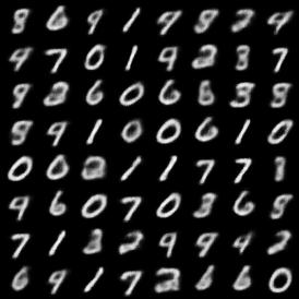
Figure 6. MNIST digit reconstruction by the convolutional variational autoencoder neural network in PyTorch after 100 epochs. The images are very clear now. Still, we can see some overlapping reconstructions like 2 & 8. May be training a bit more will help.
Figure 6 shows the image reconstructions after 100 epochs and they are much better. Except for a few digits, we are can distinguish among almost all others. But sometimes it is difficult to distinguish whether a digit is 2 or 8 (in rows 5 and 8). Still, it seems that for a variational autoencoder neural network with such small amount units per layer, it is performing really well.
Finally, let’s take a look at the .gif file that we saved to our disk. That small snippet will provide us a much better idea of how our model is reconstructing the image with each passing epoch.
Clip 1. A short clip showing the image reconstructions by the convolutional variational autoencoder in PyTorch for all the 100 epochs.
We can clearly see in clip 1 how the variational autoencoder neural network is transitioning between the images when it starts to learn more about the data. Most of the specific transitions happen between 3 and 8, 4 and 9, and 2 and 0. It is really quite amazing. This is also because the latent space in the encoding is continuous, which helps the variational autoencoder carry out such transitions.
Further Experimentations
If you want to learn a bit more and also carry out this small project a bit further, then do try to apply the same technique on the Fashion MNIST dataset. You will be really fascinated by how the transitions happen there.
Summary and Conclusion
In this tutorial, you learned about practically applying a convolutional variational autoencoder using PyTorch on the MNIST dataset. You saw how the deep learning model learns with each passing epoch and how it transitions between the digits.
If you have any suggestions, doubts, or thoughts, then please share them in the comment section. I will surely address them.
You can contact me using the Contact section. You can also find me on LinkedIn, and X.
Liked it? Take a second to support Sovit Ranjan Rath on Patreon!
Hi Edison. That should not be an issue. But if you find any implementation similar to this with lower loss, please let me know. I will check whether I can rectify something.
Hello! It seems that the tutorial is missing the sampling part. Have you generated new images from your trained VAE ?
I am suspicious of the shape of the latent space as the KLD loss is not in the same order of magnitude as the reconstruction loss. Thank you in advance
Hello Vincent. I will look into the query that you are raising.
Apart from that, the images are saved every epoch from the validation loss outputs as the model keeps learning. So, all in all, the trained weights are being used to generate the images.
Sir, sorry to bother, may I ask in line 33 self.fc1 = nn.Linear(64, 128) why you first let the feature go to 128 and then let it go back to 16, why not just from 64 to 16? In my understanding, I need to reduce the size of the data, but why increase it to 128 first?
Hello Yeyu. It’s a good question. It’s generally how convolutional autoencoders are implemented. You may try to directly use (64, 16) as well. If you get interesting results, then you may share in the comment section also.
Hi Sovit, I am trying to match the correct channels belonging to my images to your code, where my images are 128*128*35 but the image is mostly black in the background, so only in the middle of the image 28 *28 are the information of the image. The Image ist Greyscale Image. Could you give me some advice on how to adapt your code to these settings?
its a 128*128*1 but the information are in the 28*28 inside the 128*128. That mean the image is small. How could i configure the encoder and decoder in this case?
It is still a bit unclear to me. You are saying the image is 128*128*1 but the information is 28*28. Does that mean that the input to the model is 128*128*1 or 28*28?
Hello Nick. To generate new images using a trained autoencoder, you will still need an input data point to generate the latent space. So, that process will not be much different than passing an input to the validate() function and getting the output.
I am trying to replicate this for an 512x512x3 image. The ecoder part is working fine. But, as we can see from the code, the decoder part is returning a 32x32x1 tensor. What modifications will you suggest I make to the decoder part to get 512x512x3 tensor as an output, so that I can calculate the loss correctly?
Hi Shubham. It basically depends on how the decoder has been written. It’s been a long time since I wrote this post. But I think the decoder was meant for small images. Even I will have to run the code again and check how to make it work with high-resolution images.
I may need some time for that.
This website uses cookies so that we can provide you with the best user experience possible. Cookie information is stored in your browser and performs functions such as recognising you when you return to our website and helping our team to understand which sections of the website you find most interesting and useful.
Strictly Necessary Cookies
Strictly Necessary Cookie should be enabled at all times so that we can save your preferences for cookie settings.
If you disable this cookie, we will not be able to save your preferences. This means that every time you visit this website you will need to enable or disable cookies again.


Nice work ! (Please change the scrolling animation)
Thanks for the feedback Kawther. May I ask which scrolling animation are you referring to?
Thanks,That’s really helpful! I am confused about the high loss functio,dose it really work??
Hi Edison. That should not be an issue. But if you find any implementation similar to this with lower loss, please let me know. I will check whether I can rectify something.
I think you are dividing ur Loss by counter instead of dataset size
Yes Abhra. You are right. I will correct that. Thanks for pointing it out.
Hello! It seems that the tutorial is missing the sampling part. Have you generated new images from your trained VAE ?
I am suspicious of the shape of the latent space as the KLD loss is not in the same order of magnitude as the reconstruction loss. Thank you in advance
Hello Vincent. I will look into the query that you are raising.
Apart from that, the images are saved every epoch from the validation loss outputs as the model keeps learning. So, all in all, the trained weights are being used to generate the images.
Sir, sorry to bother, may I ask in line 33 self.fc1 = nn.Linear(64, 128) why you first let the feature go to 128 and then let it go back to 16, why not just from 64 to 16? In my understanding, I need to reduce the size of the data, but why increase it to 128 first?
Hello Yeyu. It’s a good question. It’s generally how convolutional autoencoders are implemented. You may try to directly use (64, 16) as well. If you get interesting results, then you may share in the comment section also.
Hi Sovit, I am trying to match the correct channels belonging to my images to your code, where my images are 128*128*35 but the image is mostly black in the background, so only in the middle of the image 28 *28 are the information of the image. The Image ist Greyscale Image. Could you give me some advice on how to adapt your code to these settings?
Hello dayo.
It is a bit unclear about your image dimensions. You are saying it is 128*128*35. Are you sure about that? Or is it 128*128*3?
Hallo Sovit.
its a 128*128*1 but the information are in the 28*28 inside the 128*128. That mean the image is small. How could i configure the encoder and decoder in this case?
It is still a bit unclear to me. You are saying the image is 128*128*1 but the information is 28*28. Does that mean that the input to the model is 128*128*1 or 28*28?
Sovit, Very nice work! After the model is trained how do you sample new images from the trained weights?
Hello Nick. To generate new images using a trained autoencoder, you will still need an input data point to generate the latent space. So, that process will not be much different than passing an input to the validate() function and getting the output.
Hello. This is an excellent tutorial.
I am trying to replicate this for an 512x512x3 image. The ecoder part is working fine. But, as we can see from the code, the decoder part is returning a 32x32x1 tensor. What modifications will you suggest I make to the decoder part to get 512x512x3 tensor as an output, so that I can calculate the loss correctly?
Hi Shubham. It basically depends on how the decoder has been written. It’s been a long time since I wrote this post. But I think the decoder was meant for small images. Even I will have to run the code again and check how to make it work with high-resolution images.
I may need some time for that.