Autoencoders in Deep Learning

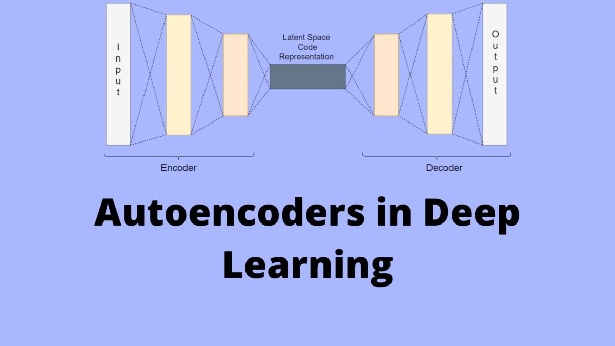
Updated: March 25, 2020.

If you are into deep learning, then till now you may have seen many cases of supervised deep learning using neural networks. In this article, we will take a dive into an unsupervised deep learning technique using neural networks. Specifically, we will learn about autoencoders in deep learning.

What Will We Cover in this Article?

– What are autoencoders?
– The principle behind autoencoders.
– Different types of autoencoders: Undercomplete autoencoders, regularized autoencoders, variational autoencoders (VAE).
– Applications and limitations of autoencoders in deep learning.

What are Autoencoders?

Autoencoders are an unsupervised learning technique that we can use to learn efficient data encodings. Basically, autoencoders can learn to map input data to the output data. While doing so, they learn to encode the data. And the output is the compressed representation of the input data.

Want to get a hands-on approach to implementing autoencoders in PyTorch? Check out this article here.

The main aim while training an autoencoder neural network is dimensionality reduction.

Quoting Francois Chollet from the Keras Blog,

“Autoencoding” is a data compression algorithm where the compression and decompression functions are 1) data-specific, 2) lossy, and 3) learned automatically from examples rather than engineered by a human.

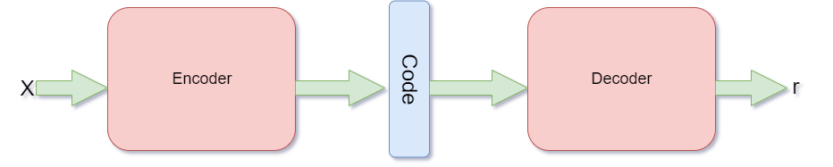
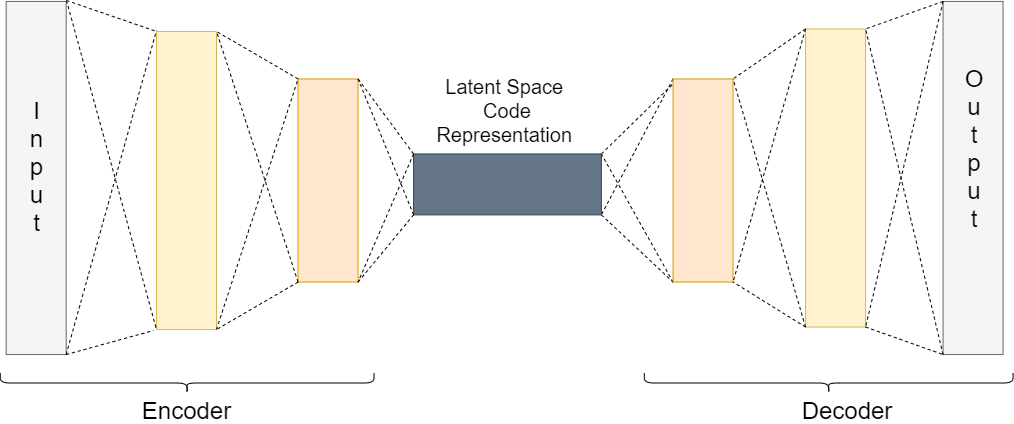
The following image shows the basic working of an autoencoder. Note that this is not a neural network specific image. It is just a basic representation of the working of the autoencoder.

Basic Principle of Autoencoder — Autoencoder

The Principle Behind Autoencoder

In an autoencoder, there are two parts, an encoder, and a decoder.

First, the encoder takes the input and encodes it. For example, let the input data be $x$. Then, we can define the encoded function as $f(x)$.

Between the encoder and the decoder, there is also an internal hidden layer. Let’s call this hidden layer $h$. This hidden layer learns the coding of the input that is defined by the encoder. So, basically after the encoding, we get $h \ = \ f(x)$.

Finally, the decoder function tries to reconstruct the input data from the hidden layer coding. If we consider the decoder function as $g$, then the reconstruction can be defined as,

$$
r = g(f(x)) \\
r = g(h)
$$

Simple Neural Network Architecture of Autoencoder

All of this is very efficiently explained in the Deep Learning book by Ian Goodfellow and Yoshua Bengio and Aaron Courville.

But while reconstructing an image, we do not want the neural network to simply copy the input to the output. This type of memorization will lead to overfitting and less generalization power.

An autoencoder should be able to reconstruct the input data efficiently but by learning the useful properties rather than memorizing it.

There are many ways to capture important properties when training an autoencoder. Let’s start by getting to know about undercomplete autoencoders.

Undercomplete Autoencoders

In the previous section, we discussed that we want our autoencoder to learn the important features of the input data. It should do that instead of trying to memorize and copy the input data to the output data.

We can do that if we make the hidden coding data to have less dimensionality than the input data. In an autoencoder, when the encoding $h$ has a smaller dimension than $x$, then it is called an undercomplete autoencoder.

The above way of obtaining reduced dimensionality data is the same as PCA. In PCA also, we try to try to reduce the dimensionality of the original data.

The loss function for the above process can be described as,

$$
L(x, r) = L(x, g(f(x)))
$$

where $L$ is the loss function. This loss function applies when the reconstruction $r$ is dissimilar from the input $x$.

Regularized Autoencoders

In undercomplete autoencoders, we have the coding dimension to be less than the input dimension.

We also have overcomplete autoencoder in which the coding dimension is the same as the input dimension. But this again raises the issue of the model not learning any useful features and simply copying the input.

One solution to the above problem is the use of regularized autoencoder. When training a regularized autoencoder we need not make it undercomplete. We can choose the coding dimension and the capacity for the encoder and decoder according to the task at hand.

To properly train a regularized autoencoder, we choose loss functions that help the model to learn better and capture all the essential features of the input data.

Next, we will take a look at two common ways of implementing regularized autoencoders.

Sparse Autoencoders

In sparse autoencoders, we use a loss function as well as an additional penalty for sparsity. Specifically, we can define the loss function as,

$$
L(x, g(f(x))) \ + \ \Omega(h)
$$

where $\Omega(h)$ is the additional sparsity penalty on the code $h$.

The following is an image showing MNIST digits. The first row shows the original images and the second row shows the images reconstructed by a sparse autoencoder.

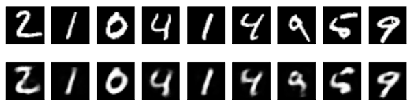
Working of Sparse Autoencoders (**Source**)

Adding a penalty such as the sparsity penalty helps the autoencoder to capture many of the useful features of data and not simply copy it.

Denoising Autoencoders

In sparse autoencoders, we have seen how the loss function has an additional penalty for the proper coding of the input data.

But what if we want to achieve similar results without adding the penalty? In that case, we can use something known as denoising autoencoder.

We can change the reconstruction procedure of the decoder to achieve that. Until now we have seen the decoder reconstruction procedure as $r(h) \ = \ g(f(x))$ and the loss function as $L(x, g(f(x)))$.

Now, consider adding noise to the input data to make it $\tilde{x}$ instead of $x$. Then the loss function becomes,

$$
L(x, g(f(\tilde{x})))
$$

The following image shows how denoising autoencoder works. The second row shows the reconstructed images after the decoder has cleared out the noise.

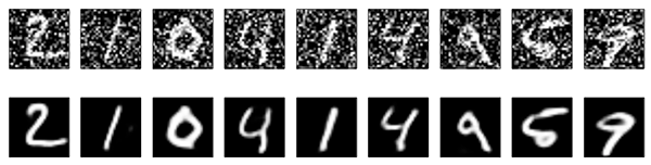
Working of Denoising Autoencoder (**Source**)

For a proper learning procedure, now the autoencoder will have to minimize the above loss function. And to do that, it first will have to cancel out the noise, and then perform the decoding.

In a denoising autoencoder, the model cannot just copy the input to the output as that would result in a noisy output. While we update the input data with added noise, we can also use overcomplete autoencoders without facing any problems.

Variational Autoencoders (VAEs)

We will take a look at a brief introduction of variational autoencoders as this may require an article of its own.

VAEs are a type of generative model like GANs (Generative Adversarial Networks).

Like other autoencoders, variational autoencoders also consist of an encoder and a decoder. But here, the decoder is the generator model. Variational autoencoders also carry out the reconstruction process from the latent code space. But in VAEs, the latent coding space is continuous.

We will take a look at variational autoencoders in-depth in a future article. In the meantime, you can read this if you want to learn more about variational autoencoders.

Applications and Limitations of Autoencoders in Deep Learning

Applications of Deep Learning Autoencoders

First, let’s go over some of the applications of deep learning autoencoders.

Dimensionality Reduction and PCA

When we use undercomplete autoencoders, we obtain the latent code space whose dimension is less than the input.

Moreover, using a linear layer with mean-squared error also allows the network to work as PCA.

Image Denoising and Image Compression

Denoising autoencoder can be used for the purposes of image denoising. Autoencoders are able to cancel out the noise in images before learning the important features and reconstructing the images.

Autoencoder can also be used for image compression to some extent. More on this in the limitations part.

Information Retrieval

When using deep autoencoders, then reducing the dimensionality is a common approach. This reduction in dimensionality leads the encoder network to capture some really important information

Limitations of Autoencoders

We have seen how autoencoders can be used for image compression and reconstruction of images. But in reality, they are not very efficient in the process of compressing images. Also, they are only efficient when reconstructing images similar to what they have been trained on.

Due to the above reasons, the practical usages of autoencoders are limited. But still learning about autoencoders will lead to the understanding of some important concepts which have their own use in the deep learning world.

Summary and Conclusion

I hope that you learned some useful concepts from this article. In future articles, we will take a look at autoencoders from a coding perspective. If you have any queries, then leave your thoughts in the comment section. I will try my best to address them.

You can find me on LinkedIn and Twitter as well.

Liked it? Take a second to support Sovit Ranjan Rath on Patreon!