Machine Learning Hands-On: Convolutional Autoencoders

Updated: March 25, 2020.

Convolutional autoencoders are some of the better know autoencoder architectures in the machine learning world. In this article, we will get hands-on experience with convolutional autoencoders. For implementation purposes, we will use the PyTorch deep learning library.

What Will We Cover in this Article?

• Implementing convolutional autoencoders using PyTorch.
• Visualizing and comparing the original and reconstructed images during the learning procedures of the neural network.

If you want to get some background knowledge about deep learning autoencoders, then you can read this article.

Also, to get coding knowledge of autoencoders in deep learning, you can visit my previous article – Implementing Deep Autoencoder in PyTorch.

What Dataset Will We be Using?

It is common practice to use the MNIST or the Fashion MNIST dataset for an easier understanding of deep learning concepts. But will use the CIFAR10 dataset in this article. This will provide us enough challenges to tackle and learn more at the same time. Also, we will get to know how to work with colored images in deep learning autoencoders.

Background About the CIFAR10 Dataset

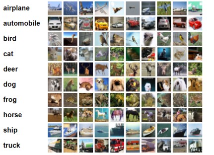
The CIFAR10 dataset contains 60000 32×32 colored images. The dataset is divided into 10 classes with 6000 images per class, with 50000 training images and 10000 test images.

If you want to know about the dataset in-depth, then you can visit the CIFAR10 page by Alex Krizhevsky.

We are now all set to start implementing our first autoencoder architecture – Convolutional Autoencoder.

Convolutional Autoencoder on the CIFAR10 Dataset.

Let’s start by importing all the required libraries and modules.

import os
import torch 
import torchvision
import torch.nn as nn
import torchvision.transforms as transforms
import torch.optim as optim
import torch.nn.functional as F
import matplotlib.pyplot as plt

from torchvision import datasets
from torch.utils.data import DataLoader
from torchvision.utils import save_image

The imported modules include:

• torchvision: contains many popular computer vision datasets, deep neural network architectures, and image processing modules. We will use this to download the CIFAR10 dataset.
• torch.nn: contains the deep learning neural network layers such as Linear(), and Conv2d().
• transforms: will help in defining the image transforms and normalizations.
• optim: contains the deep learning optimizer classes such as MSELoss()and many others as well.
• functional: we will use this for activation functions such as ReLU.
• DataLoader: eases the task of making iterable training and testing sets.

Defining the Constants

We should define the constants beforehand so that we can use them whenever required. We will be defining the number of epochs, the batch size, and the learning rate.

NUM_EPOCHS = 50
LEARNING_RATE = 1e-3
BATCH_SIZE = 32

So, we have the number of epochs as 50, the learning rate is 0.001, and the batch size is 32.

Preparing the Data

Here, we will define the data image transformations for the CIFAR10 images. Also, we will download the data using torchvision.datasets. Then we will use the Dataloader module to prepare the training and test set.

First, let’s define the image transforms. For that, we will use torchvision.transforms.

transform = transforms.Compose([
    transforms.ToTensor(),
    transforms.Normalize((0.5, 0.5, 0.5), (0.5, 0.5, 0.5))
])

In the above code block, we are converting the data into torch tensors and normalizing the data.

After defining the transforms we can prepare our data and apply the transforms.

trainset = datasets.CIFAR10(
    root='./data',
    train=True, 
    download=True,
    transform=transform
)
testset = datasets.CIFAR10(
    root='./data',
    train=False,
    download=True,
    transform=transform
)

trainloader = DataLoader(
    trainset, 
    batch_size=BATCH_SIZE,
    shuffle=True
)
testloader = DataLoader(
    testset, 
    batch_size=BATCH_SIZE, 
    shuffle=True
)

The above code will download the CIFAR10 data if you do not already have it. After downloading the data, you should see a data directory containing the CIFAR10 dataset.

Some Helper Functions

In this section, we will define some helper functions that will make our work easier along the way. We will get to explanation after defining the code.

def get_device():
    if torch.cuda.is_available():
        device = 'cuda:0'
    else:
        device = 'cpu'
    return device

def make_dir():
    image_dir = 'Conv_CIFAR10_Images'
    if not os.path.exists(image_dir):
        os.makedirs(image_dir)

def save_decoded_image(img, name):
    img = img.view(img.size(0), 3, 32, 32)
    save_image(img, name)

We have three functions in the above code snippet. Let’s take a look at each of them.

• get_device(): this function returns the computation device. That is, it will return either the CUDA GPU device if present, or the CPU.
• make_dir(): this will make a directory named Conv_CIFAR10_Images. We will save the original and decoded images in this directory while training the neural network.
• save_decoded_image(): this is a very simple function that will save the images in the Conv_CIFAR10_Images directory.

Defining the Autoencoder Neural Network

Next, we will define the convolutional autoencoder neural network. This is a very simple neural network. Unlike other really big and deep neural networks, ours is going to be only four layers deep.

The following is the Autoencoder() class defining the autoencoder neural network.

class Autoencoder(nn.Module):
    def __init__(self):
        super(Autoencoder, self).__init__()

        # encoder
        self.enc1 = nn.Conv2d(
            in_channels=3, out_channels=8, kernel_size=3
        )
        self.enc2 = nn.Conv2d(
            in_channels=8, out_channels=4, kernel_size=3
        )

        # decoder 
        self.dec1 = nn.ConvTranspose2d(
            in_channels=4, out_channels=8, kernel_size=3
        )
        self.dec2 = nn.ConvTranspose2d(
            in_channels=8, out_channels=3, kernel_size=3
        )

    def forward(self, x):
       x = F.relu(self.enc1(x))
       x = F.relu(self.enc2(x))
       x = F.relu(self.dec1(x))
       x = F.relu(self.dec2(x))
       return x

net = Autoencoder()
print(net)

Within the __init__() function, we first have two 2D convolutional layers (lines 6 to 11). The in_channels and out_channels are 3 and 8 respectively for the first convolutional layer. The second convolutional layer has 8 in_channels and 4 out_channles. These two nn.Conv2d() will act as the encoder. After taking the pixel data as input, they will produce the hidden code from it. Then this hidden code will be given as input to the decoder to again reconstruct the images.

Coming to the decoder part of the autoencoder. Again we have two ConvTranspose2d(). Both of these have the in_channels and out_channels in the reverse order of the Conv2d(). They take the latent space code and try to decode. This decoding process results in the return of initial pixel values that were given as input to the encoder.

In the forward() method we have stacked our neural network layers with the ReLU activation function. Finally, we return the autoencoder network. Then we define a net object for the autoencoder network.

Define the Loss Function and the Optimizer

We will use MSELoss() as the loss function and the Adam optimizer.

criterion = nn.MSELoss()
optimizer = optim.Adam(net.parameters(), lr=LEARNING_RATE)

Define the Training and Test Functions

In this section, we will define the functions to train and test our autoencoder neural network.

def train(net, trainloader, NUM_EPOCHS):
    train_loss = []
    for epoch in range(NUM_EPOCHS):
        running_loss = 0.0
        for data in trainloader:
            img, _ = data # no need for the labels
            img = img.to(device)
            optimizer.zero_grad()
            outputs = net(img)
            loss = criterion(outputs, img)
            loss.backward()
            optimizer.step()
            running_loss += loss.item()
        
        loss = running_loss / len(trainloader)
        train_loss.append(loss)
        print('Epoch {} of {}, Train Loss: {:.3f}'.format(
            epoch+1, NUM_EPOCHS, loss))

        if epoch % 5 == 0:
            save_decoded_image(img.cpu().data, name='./Conv_CIFAR10_Images/original{}.png'.format(epoch))
            save_decoded_image(outputs.cpu().data, name='./Conv_CIFAR10_Images/decoded{}.png'.format(epoch))

    return train_loss

def test_image_reconstruction(net, testloader):
     for batch in testloader:
        img, _ = batch
        img = img.to(device)
        outputs = net(img)
        outputs = outputs.view(outputs.size(0), 3, 32, 32).cpu().data
        save_image(outputs, 'conv_cifar10_reconstruction.png')
        break

The train() function takes the neural network object (net), the trainloader, and the number of epochs as the input arguments. Also, you can observe at line 6 that we are not extracting the image labels as we do not need them for training the autoencoder neural network. We are printing the loss values after each epoch, and saving the original image batch and the decoded batch after every 5 epochs (lines 20 to 23). The function returns the train_loss list with all the losses for the 50 epochs.

The test() function is almost the same except we are not backpropagating the gradients. Also, notice that we are only reconstructing the images for a single batch only, not the whole test dataloader.

We have all the code in place. Now, we just need to call each of the functions and plot the loss values to see how our model performs.

device = get_device()
print(device)
net.to(device)
make_dir()
train_loss = train(net, trainloader, NUM_EPOCHS)
plt.figure()
plt.plot(train_loss)
plt.title('Train Loss')
plt.xlabel('Epochs')
plt.ylabel('Loss')
plt.savefig('conv_ae_cifar10_loss.png')
test_image_reconstruction(net, testloader)

Epoch 1 of 50, Train Loss: 0.158
Epoch 2 of 50, Train Loss: 0.146
Epoch 3 of 50, Train Loss: 0.145
Epoch 4 of 50, Train Loss: 0.144
Epoch 5 of 50, Train Loss: 0.144
...
Epoch 45 of 50, Train Loss: 0.143
Epoch 46 of 50, Train Loss: 0.143
Epoch 47 of 50, Train Loss: 0.143
Epoch 48 of 50, Train Loss: 0.143
Epoch 49 of 50, Train Loss: 0.143
Epoch 50 of 50, Train Loss: 0.143

Analyzing the Loss Plot

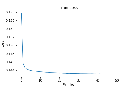
Our model seems to be performing well. But still, after the first few epochs, the loss values tend to decrease very slowly.

We will get more information on the performance of the network after we see the original and reconstructed images.

The following two images show the original and decoded images after 25 training epochs.

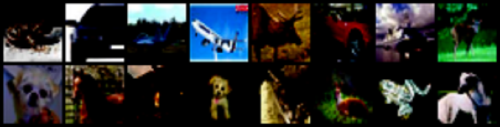
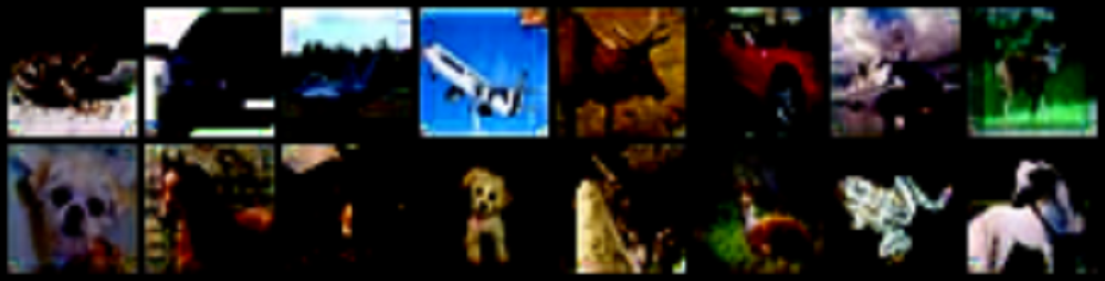
The first image shows the original image and the second one shows the decoded image. Although both of them look the same, they have very subtle differences that are not visible very clearly. There is some loss in pixel information as well as some noise in some of the images if you look really closely. But most of the time we will not notice them.

Overall, our network seems to be performing really well. But still, if you want, you can try and add pooling layers into the network and see how it performs. Maybe adding pooling layers will cause the loss values to decrease more with the number of epochs.

Want More Machine Learning and Deep Learning Concepts?

I write deep learning and machine learning posts each week and try to improve with every new post. If you want you can take a look at all the posts and learn even more.

Summary and Conclusion

If you found the article helpful, then share this with others. You can comment on any inconsistencies in the code and concepts in the comment section or reach me directly using the contacts.

You can also find me on LinkedIn, and Twitter.