Implementing Deep Autoencoder in PyTorch

Updated on 14 November 2020.

In this article, we take a hands-on approach to building deep learning autoencoders. We will implement deep autoencoders using linear layers with PyTorch.

What Will We Cover in this Article?

• A brief introduction to autoencoders.
• The approach for this article.
• Building a deep autoencoder with PyTorch linear layers.
• We will also take a look at all the images that are reconstructed by the autoencoder for better understanding.

A Brief Introduction to Autoencoders

Deep learning autoencoders are a type of neural network that can reconstruct specific images from the latent code space.

The autoencoders obtain the latent code data from a network called the encoder network. Then we give this code as the input to the decoder network which tries to reconstruct the images that the network has been trained on.

The following image summarizes the above theory in a simple manner.

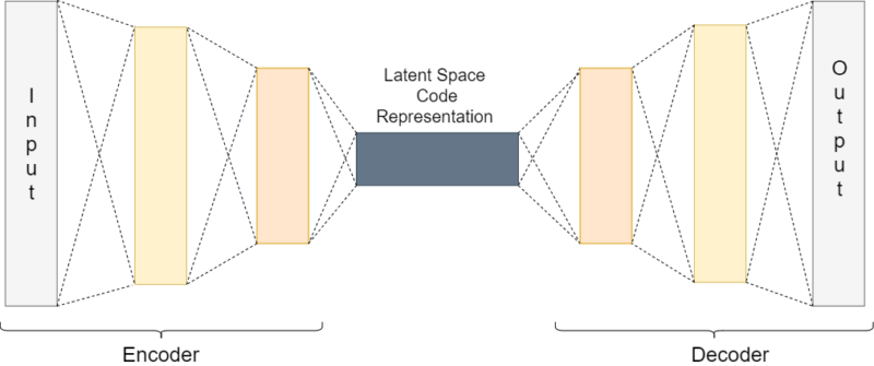
The above image summarizes the working of an autoencoder, be it a deep or convolutional autoencoder.

In one of my previous articles, I have covered the basics of autoencoder in deep learning. You can read the article here (Autoencoders in Deep Learning).

What Approach Will We be Taking?

So, we will carry out a baseline project with PyTorch in this article. This project should be enough for any newcomer to understand the working of deep autoencoders and to carry out further experimentations.

We will train a deep autoencoder using PyTorch Linear layers. For this one, we will be using the Fashion MNIST dataset. This is will help to draw a baseline of what we are getting into with training autoencoders in PyTorch.

In future articles, we will implement many different types of autoencoders using PyTorch. Specifically, we will be implementing deep learning convolutional autoencoders, denoising autoencoders, and sparse autoencoders.

Deep Autoencoder using the Fashion MNIST Dataset

Let’s start by building a deep autoencoder using the Fashion MNIST dataset.

The Fashion MNIST dataset has proven to be very useful for many baseline benchmarks in deep learning projects, algorithms, and ideas. Although, it is a very simple dataset, yet we will be able to learn a lot of underlying concepts of deep learning autoencoders using the dataset. So, let’s get started.

I hope that you are aware of the Fashion MNIST dataset. Still, to give a bit of perspective, the dataset contains 70000 grayscale images of fashion items and garments. The dataset is divided into a train set of 60000 images and a test set of 10000 images. The images belong to 10 classes, 0: t-shirt/top, 1: trouser, 2: pullover, 3: dress, 4: coat, 5: sandal, 6: shirt, 7: sneaker, 8: bag, 9: ankle boot.

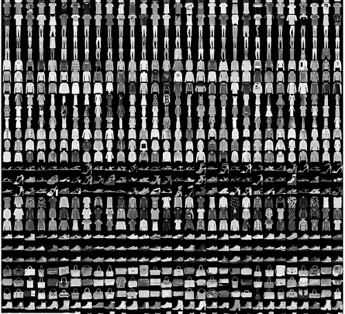
You can read more about the dataset here.

You can either use Jupyter Notebook or any IDE that you are comfortable with. I have tried my best to keep the code compatible with both notebook and IDE environments. Still, if you find any inconsistencies in the code, then feel free to reach up to me either in the comment section or through the contacts.

Okay, we are all set to start writing our code. You can either copy/paste and run the code, or write along with the article.

Importing the Required Libraries and Modules

First, let’s import all the required libraries and modules for the project.

# import packages
import os
import torch 
import torchvision
import torch.nn as nn
import torchvision.transforms as transforms
import torch.optim as optim
import matplotlib.pyplot as plt
import torch.nn.functional as F
 
from torchvision import datasets
from torch.utils.data import DataLoader
from torchvision.utils import save_image

Some of the important imports include:

• – torchvision: contains many popular computer vision datasets, deep neural network architectures, and image processing modules. We will use this to download the Fashion MNIST and in later articles the CIFAR10 dataset as well.
• – torch.nn: contains the deep learning neural network layers such as Linear(), and Conv2d().
• – transforms: will help in defining the image transforms and normalizations.
• – optim: contains the deep learning optimizer classes such as MSELoss()and many others as well.
• – functional: we will use this for activation functions such as ReLU.
• – DataLoader: eases the task of making iterable training and testing sets.

If you get confused while using the imports, always remember to check the official PyTorch docs. They are really helpful in understanding many of the things.

Define Constants and Prepare the Data

In this section, we will define some constants that we will need along the way. Also, we will prepare the dataset. If you already do not have the dataset in your current working directory, then it will be downloaded first.

Let’s begin by defining our constants and also the image transformations.

# constants
NUM_EPOCHS = 50
LEARNING_RATE = 1e-3
BATCH_SIZE = 128

# image transformations
transform = transforms.Compose([
    transforms.ToTensor(),
])

The first three lines in the above code block define the constants, the number of epochs, the learning rate, and the batch size for images. A batch size of 128 for Fashion MNIST should not cause any problem. Still, if you get OOM (Out Of Memory Error), then try reducing the size to 64 or 32.

From line 6, we define the image transformations. Basically, we are converting the pixel values to tensors first which is the best form to use any data in PyTorch. Next, we are normalizing the pixel values so that they will fall in the range of [-1, 1].

Now, let’s prepare the training and testing data. PyTorch makes it really easy to download and convert the dataset into iterable data loaders.

trainset = datasets.FashionMNIST(
    root='./data',
    train=True, 
    download=True,
    transform=transform
)
testset = datasets.FashionMNIST(
    root='./data',
    train=False,
    download=True,
    transform=transform
)

trainloader = DataLoader(
    trainset, 
    batch_size=BATCH_SIZE,
    shuffle=True
)
testloader = DataLoader(
    testset, 
    batch_size=BATCH_SIZE, 
    shuffle=True
)

So, we are applying the transforms to the images that we have defined before. The trainloader and testloader each is of batch size 128. The data loaders are iterable and you will be able to iterate through them till the number of batches in them. Specifically, the trainloader contains 60000/128 number of batches, and the testloader contains 10000/128 number of batches.

Utility Functions

It is always better to write some utility functions. This would save time and also avoid code repetition. Below are three utility functions that we will need along the way.

# utility functions
def get_device():
    if torch.cuda.is_available():
        device = 'cuda:0'
    else:
        device = 'cpu'
    return device

def make_dir():
    image_dir = 'FashionMNIST_Images'
    if not os.path.exists(image_dir):
        os.makedirs(image_dir)

def save_decoded_image(img, epoch):
    img = img.view(img.size(0), 1, 28, 28)
    save_image(img, './FashionMNIST_Images/linear_ae_image{}.png'.format(epoch))

The first function, get_device() either returns the GPU device if it is available or the CPU. If you notice, this is a bit different from the one-liner code used in the PyTorch tutorials. This is because some IDEs do not recognize the torch.device() method. Therefore, to keep the code compatible for both IDE and python notebooks I just changed the code a bit.

The second function is make_dir() which makes a directory to store the reconstructed images while training. At last, we have save_decoded_image() which saves the images that the autoencoder reconstructs.

Define the Autoencoder Network

In this section, we will define the autoencoder network. Let’s define the network first, then we will get to the code explanation.

class Autoencoder(nn.Module):
    def __init__(self):
        super(Autoencoder, self).__init__()

        # encoder
        self.enc1 = nn.Linear(in_features=784, out_features=256)
        self.enc2 = nn.Linear(in_features=256, out_features=128)
        self.enc3 = nn.Linear(in_features=128, out_features=64)
        self.enc4 = nn.Linear(in_features=64, out_features=32)
        self.enc5 = nn.Linear(in_features=32, out_features=16)

        # decoder 
        self.dec1 = nn.Linear(in_features=16, out_features=32)
        self.dec2 = nn.Linear(in_features=32, out_features=64)
        self.dec3 = nn.Linear(in_features=64, out_features=128)
        self.dec4 = nn.Linear(in_features=128, out_features=256)
        self.dec5 = nn.Linear(in_features=256, out_features=784)

    def forward(self, x):
        x = F.relu(self.enc1(x))
        x = F.relu(self.enc2(x))
        x = F.relu(self.enc3(x))
        x = F.relu(self.enc4(x))
        x = F.relu(self.enc5(x))

        x = F.relu(self.dec1(x))
        x = F.relu(self.dec2(x))
        x = F.relu(self.dec3(x))
        x = F.relu(self.dec4(x))
        x = F.relu(self.dec5(x))
        return x

net = Autoencoder()
print(net)

Inside the Autoencoder() class we have an encoder part and a decoder part. First, the encoder takes the flattened pixel features (28×28 = 784). We define five Linear() layers until the final out_features are 16 (line 10). The encoder produces the latent code representation which then goes to the decoder for reconstruction.

Next, we have the decoder, which again keeps increasing the feature size until we get the original 784 pixels as out_features (line 18).

The forward() method simply combines the encoder and decoder with the ReLU activation function after each layer. Finally, the forward() method returns the network.

At line 33 we create a net instance of Autoencoder() class and we can refer to it whenever we need to use the neural network.

Actually, we do not even need such a large network for the Fashion MNIST dataset. Even two linear layers can effectively capture all the important features of the images. Be sure to try that on your own and share the results in the comment section.

Defining, the loss function and the optimizer for our network:

criterion = nn.MSELoss()
optimizer = optim.Adam(net.parameters(), lr=LEARNING_RATE)

Train and Test Functions

Let’s define the train and test functions that we will be using.

def train(net, trainloader, NUM_EPOCHS):
    train_loss = []
    for epoch in range(NUM_EPOCHS):
        running_loss = 0.0
        for data in trainloader:
            img, _ = data
            img = img.to(device)
            img = img.view(img.size(0), -1)
            optimizer.zero_grad()
            outputs = net(img)
            loss = criterion(outputs, img)
            loss.backward()
            optimizer.step()
            running_loss += loss.item()
        
        loss = running_loss / len(trainloader)
        train_loss.append(loss)
        print('Epoch {} of {}, Train Loss: {:.3f}'.format(
            epoch+1, NUM_EPOCHS, loss))

        if epoch % 5 == 0:
            save_decoded_image(outputs.cpu().data, epoch)

    return train_loss

def test_image_reconstruction(net, testloader):
     for batch in testloader:
        img, _ = batch
        img = img.to(device)
        img = img.view(img.size(0), -1)
        outputs = net(img)
        outputs = outputs.view(outputs.size(0), 1, 28, 28).cpu().data
        save_image(outputs, 'fashionmnist_reconstruction.png')
        break

There are some key points to notice inside the train() function. At line 6 we are only extracting the image pixels data as we do not the labels to train the autoencoder network. As we are using linear layers, at line 8 we are flattening the image pixels to tensors of 784 dimensions. After each epoch, we are appending the loss values to the train_loss list which we are returning at the end of the function. Also, every 5 epochs, we are saving the reconstructed images. This gives us a proper idea of how well our neural network is actually performing.

Inside the test_image_reconstruction() function we are just reconstructing a single batch of the image from our testloader. You can reconstruct the images for all the batches if you like.

Training the Autoencoder Network

Here, we will call the utility functions, and train and test our network.

# get the computation device
device = get_device()
print(device)
# load the neural network onto the device
net.to(device)

make_dir()

# train the network
train_loss = train(net, trainloader, NUM_EPOCHS)
plt.figure()
plt.plot(train_loss)
plt.title('Train Loss')
plt.xlabel('Epochs')
plt.ylabel('Loss')
plt.savefig('deep_ae_fashionmnist_loss.png')

# test the network
test_image_reconstruction(net, testloader)

First, we get the computation device (line 2). Next, we load our deep neural network onto the device (line 5). Then we make the directory to store the reconstructed images.

After training the network for 50 epochs line 10, we save the loss plot on the disk. Finally, we call test_image_reconstruction() (line 19) to test our network on a single batch of images.

Autoencoder(
  (enc1): Linear(in_features=784, out_features=256, bias=True)
  (enc2): Linear(in_features=256, out_features=128, bias=True)
  (enc3): Linear(in_features=128, out_features=64, bias=True)
  (enc4): Linear(in_features=64, out_features=32, bias=True)
  (enc5): Linear(in_features=32, out_features=16, bias=True)
  (dec1): Linear(in_features=16, out_features=32, bias=True)
  (dec2): Linear(in_features=32, out_features=64, bias=True)
  (dec3): Linear(in_features=64, out_features=128, bias=True)
  (dec4): Linear(in_features=128, out_features=256, bias=True)
  (dec5): Linear(in_features=256, out_features=784, bias=True)
)
cuda:0
Epoch 1 of 50, Train Loss: 0.652
Epoch 2 of 50, Train Loss: 0.638
Epoch 3 of 50, Train Loss: 0.632
Epoch 4 of 50, Train Loss: 0.630
Epoch 5 of 50, Train Loss: 0.628
...
Epoch 46 of 50, Train Loss: 0.611
Epoch 47 of 50, Train Loss: 0.611
Epoch 48 of 50, Train Loss: 0.611
Epoch 49 of 50, Train Loss: 0.611
Epoch 50 of 50, Train Loss: 0.611

Analyzing Plots and Image Reconstructions

From the training, you must have noticed that the loss values decrease very slowly after the first 10 epochs. Now, let’s look at the saved loss plot once.

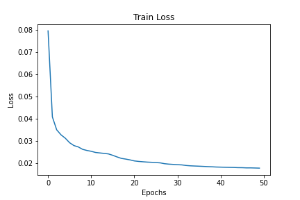
By the end of 50 epochs are achieving a loss value of around 0.611.

To get an even better perspective, let’s look at three of the image training reconstructions.

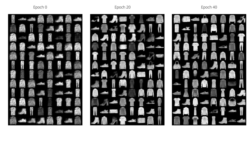
We can see that, at the very beginning, the decoder network reconstructions are not complete. But by the end of 40 epochs the neural network has learned to reconstruct most of the images from the latent code representation. You should try training a smaller network and see the results that you get.

Summary and Conclusion

This post is a bit long for a single deep autoencoder implementation with PyTorch. However, in deep learning, if you understand even a single concept clearly, then the related concepts become easier to understand. I hope that you learned how to implement deep autoencoder in deep learning with PyTorch. If you have any queries, you can post it in the comment section. Share this article with others if you think that others might as well benefit from it.

In the next article, we will be implementing convolutional autoencoders in PyTorch.

You can find me on LinkedIn, and Twitter.