In this tutorial, we will be doing something really interesting, fun, and containing a lot of learning as well. We will use deep learning and PyTorch to train a convolutional variational autoencoder neural network which will generate colored images. And not just any colored images. The neural network will be generating faces of fictional celebrities. So, in specific, we will be generating fictional celebrity faces using convolutional variational autoencoder and PyTorch.
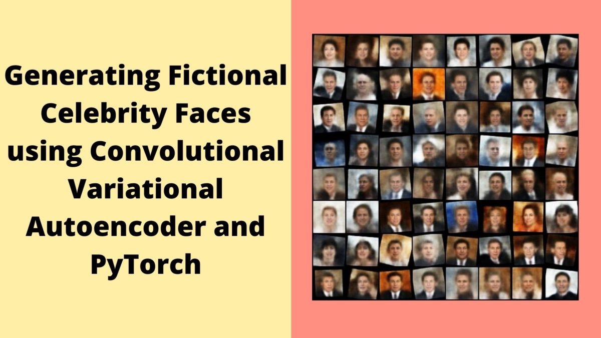
If you want a sneak peek of what results we will actually get in this tutorial, well, here it is.
Figure 1. Fictional celebrity faces generated by a convolutional variational autoencoder. You can expect to get similar results after going through this tutorial.
If you are searching for some well-known faces in figure 1, most probably, you won’t find them. Reason being, we only want to train our convolutional variational autoencoder neural network model on celebrity images. After that it should be able to generate new and unseen celebrity faces. Also, we won’t be trying to generate very high resolution images. There are two reasons for this.
I want this tutorial to be accessible to everybody with reasonable computation time.
Generative Adversarial Networks (GANs) are much better at outputting high-resolution images.
So, what will you be learning in specific?
Creating a convolutional variational autoencoder model that is good at generating images.
We will train the deep learning model on the Labelled Faces in the Wild (LFW) Dataset dataset from Kaggle. Because it is small in size, around 112 MB. Still, it contains over 13000 images. This means that it will provide our convolutional variational autoencoder neural network with enough images to learn from.
During the validation step, we will try to generate new and fictional celebrity faces using our autoencoder neural network.
Before Moving Further…
I keep a section like this in almost all of my autoencoder posts. If you are new to autoencoders in general, then please take a look at the following posts before moving further.
Autoencoders in Deep Learning: This will give you a very short and general introduction to autoencoders in deep learning in general.
And if you just want to get started with convolutional variational autoencoder, then this article will be the perfect place to get an idea. In the article, you will know how to prepare an error-free convolutional variational autoencoder model. Along with that, you will train the autoencoder neural network on MNIST images to generate new digits. It is the perfect place if you are new to convolutional variational autoencoders.
Note: I try my best to keep all my articles error-free. Still, some sort of errors may creep into the articles. Autoencoders are a somewhat tricky area in deep learning and neural networks. Combining theory and concepts into a short blog tutorial may contain errors. If you find any errors or discrepancies, be it in theory or coding, then please feel free to reach out either through the comment section or contact section.
I hope that you are excited to move along with me into this tutorial.
Libraries and Frameworks that We Will be Using
The most important framework for this tutorial is PyTorch. All the code in this tutorial, are based on PyTorch version 1.6. Earlier and newer versions should not cause any issue as well. If you have not installed PyTorch on your system, you can easily do it from here.
Directory Structure and Dataset
We will follow the below given directory structure for this tutorial.
The input folder contains the dataset that we will use to train the autoencoder neural network model. We will know more about that shortly.
The outputs folder will contain all the image reconstructions by the deep learning model and the loss plot for training and validation. It will also contain a GIF file that will showcase the image reconstructions by the variational autoencoder through all the epochs.
Finally, the src folder contains six of the Python scripts that we will code through. Yes, I know, these are a lot of scripts. But stick till the end, and you will surely get amazing results.
Coming to the dataset. We will be using the Labelled Faces in the Wild (LFW) Dataset from Kaggle. This contains around 5000 folders with images of many well-known celebrities. Some folders contain multiple images. The total images amount to more than 13000. These should be enough to train a reasonably good variational autoencoder capable of generating new celebrity faces. The dataset also contains many labels in CSV file format. But we will not be needing those. We can ignore them as we will be working with the images only.
Download the dataset and extract it inside the input folder to get the directory structure as above.
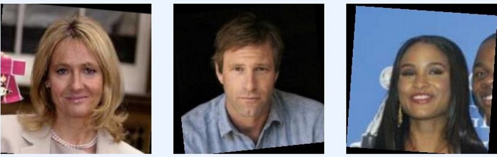
To get an idea of the images that the dataset provides, here are a few.
Figure 2. Examples of a few celebrity faces from the LFW dataset. We will train our convolutional variational autoencoder model on these images.
Figure 2 shows a few celebrity images to just get an idea of the images that the dataset contains.
Now, that all the preliminary things are done, let’s jump directly into the coding part of the tutorial.
Generating Fictional Celebrity Faces using Convolutional Variational Autoencoder and PyTorch
From this section onward, we will start to write the code for generating fictional celebrity faces using convolutional variational autoencoder and PyTorch.
The first step is going to be preparing the dataset. Let’s start with that.
Prepare the Data from the Image Folders
You must have observed that the images are in the several folders nested inside the root dataset folder. We need to extract all the image files before we can move further with writing out dataset class to return the image batches.
Open up the prepare_data.py script inside the src folder and write the following code in there.
import glob as glob
import os

from tqdm import tqdm

def prepare_dataset(ROOT_PATH):
    image_dirs = os.listdir(ROOT_PATH)
    image_dirs.sort()
    print(len(image_dirs))
    print(image_dirs[:5])

    all_image_paths = []

    for i in tqdm(range(len(image_dirs))):
        image_paths = glob.glob(f"{ROOT_PATH}/{image_dirs[i]}/*")
        image_paths.sort()
        for image_path in image_paths:
            all_image_paths.append(image_path)


    print(f"Total number of face images: {len(all_image_paths)}")

    train_data = all_image_paths[:-2000]
    valid_data = all_image_paths[-2000:]

    print(f"Total number of training image: {len(train_data)}")
    print(f"Total number of validation image: {len(valid_data)}")
    return train_data, valid_data
We have a prepare_dataset() function that accepts the ROOT_PATH to the dataset as a parameter.
We keep all the folder paths in a image_dirs list and sort it alphabetically.
Starting from line 14, we loop over the number of folders in image_dirs.
We extract the image paths from each of the folder paths and keep on appending those image paths to the all_image_paths list. We have defined this list at line 12.
Lines 23 and 24 divide the data into train_data and valid_data. We will be using the last 2000 images for validation and the rest for training.
Then we are just printing some information on the screen and returning the train_data and valid_data.
If you have limited computing power, then do consider using fewer images for training and validation. You just need to change the slicing values for train_data and valid_data in the above code block. Choose whatever value works best for you. According to the above code, we have around 11000 images for training and 2000 images for validation.
Prepare the PyTorch Dataset
Here, we will write a PyTorch dataset class that will return us the batches of images. If you work with PyTorch regularly, then you must have done this several times before for image datasets.
All the code here will go into the dataset.py script inside the src folder. The following is the LFWDataset() that prepares our image data to be fed into a neural network.
The __init__() function accepts data_list and transform as parameters. We are initializing those two at lines 7 and 8.
The data_list is either going to be train_data or valid_data that we have in the above section.
The __len__() function just returns the number of instances when called.
Inside the __getitem__() function, first we are reading the image using OpenCV at line 14.
All of the original images are 250×250 in dimension. But we will not be training such large images. Using around 11000 images with such large dimensions for training will demand a lot of training time and compute power. We can get reasonable quality and training time if we can reduce the image dimensions. Therefore, we are resizing all the images to 64×64 at line 15. Line 16 converts the BGR color format images to RGB format.
Then we apply the image transforms and finally return the image.
That’s it for the PyTorch dataset class. Further, we will be writing some utility functions that will handle some simple and repetitive tasks for us.
Writing some Utility Functions
Every project has some code or functions that are repetitive and can be kept somewhat separate from other codes. We can keep such code in a utils.py script and just call them when we need them.
We will be writing a few such lines of code here. All of the utility code will go into the utils.py script inside the src folder.
The following are the imports that we need for our utility script.
import imageio
import numpy as np
import torchvision.transforms as transforms
import matplotlib.pyplot as plt

from torchvision.utils import save_image
One of the important imports here is imageio. We need this to save our output reconstructions images as GIF file. We will get to that a bit later.
Define the Image Transforms
We need a few PyTorch image transform code. Let’s write the code first, then we will get into the explanation part.
First, we have the to_pil_image that transforms an image tensor to PIL image format. This we need for converting all the output image tensors so that we can save them as a GIF file. I hope that this part is clear.
Then starting from line 9, we have a transform() function. This just converts the NumPy array images to PyTorch tensors and nothing more. We will be using this while preparing our LFWDataset(). These are the image transforms that we apply there.
The Rest of the Utility Functions
The following block of code defines the rest of the utility functions that we will need along the way.
We have the image_to_vid() function at line 14. This accepts images parameter which is a grid of reconstructed image tensors. It saves those images as a GIF file to the disk. This means that we will have a short video of all the image reconstructions through all the training epochs. It will be quite fun to watch that.
The save_reconstructed_images() function at line 18 saves the reconstruction images to the disk. These reconstructions are nothing but the output from the convolutional variational autoencoder that we will be training a bit further on.
At line 21 we have the save_loss_plot() function that saves the training and validation line plots to the disk.
The above are all the utility code that we need along the way. The next step is writing the code to prepare the convolutional variational autoencoder model.
Preparing The Convolutional Variational Autoencoder Deep Learning Model using PyTorch
In this section, we will write the code for preparing our autoencoder deep learning neural network model.
Having a good autoencoder architecture is almost always the key to get good image reconstructions in the outputs. We will try our best to prepare a good model.
Before moving further. We will not go into much detail about the explanation of the architecture of the autoencoder deep learning model here. The reason being, I have already provided a detailed explanation in the previous post here. In that tutorial, we are training a very similar convolutional variational autoencoder model on the MNIST dataset. There are only very few and minor differences. Likes the image color channels which affect the output and input channels of the model. Some other changes are the number of filters and features for convolutional and linear layers. I hope that these are pretty self-explanatory.
We will write the deep learning model code inside the model.py script in the src folder.
The following code block contains the whole of the autoencoder neural network model code.
import torch
import torch.nn as nn
import torch.nn.functional as F

init_channels = 64 # initial number of filters
image_channels = 3 # color channels

latent_dim = 100 # number of features to consider

# define a Conv VAE
class ConvVAE(nn.Module):
    def __init__(self):
        super(ConvVAE, self).__init__()

        # encoder
        self.enc1 = nn.Conv2d(
            in_channels=image_channels, out_channels=init_channels,
            kernel_size=4, stride=2, padding=2
        )
        self.enc2 = nn.Conv2d(
            in_channels=init_channels, out_channels=init_channels*2,
            kernel_size=4, stride=2, padding=2
        )
        self.enc3 = nn.Conv2d(
            in_channels=init_channels*2, out_channels=init_channels*4,
            kernel_size=4, stride=2, padding=2
        )
        self.enc4 = nn.Conv2d(
            in_channels=init_channels*4, out_channels=init_channels*8,
            kernel_size=4, stride=2, padding=2
        )
        self.enc5 = nn.Conv2d(
            in_channels=init_channels*8, out_channels=1024,
            kernel_size=4, stride=2, padding=2
        )

        self.fc1 = nn.Linear(1024, 2048)
        self.fc_mu = nn.Linear(2048, latent_dim)
        self.fc_log_var = nn.Linear(2048, latent_dim)
        self.fc2 = nn.Linear(latent_dim, 1024)

        # decoder
        self.dec1 = nn.ConvTranspose2d(
            in_channels=1024, out_channels=init_channels*8,
            kernel_size=3, stride=2
        )
        self.dec2 = nn.ConvTranspose2d(
            in_channels=init_channels*8, out_channels=init_channels*4,
            kernel_size=3, stride=2
        )
        self.dec3 = nn.ConvTranspose2d(
            in_channels=init_channels*4, out_channels=init_channels*2,
            kernel_size=3, stride=2
        )
        self.dec4 = nn.ConvTranspose2d(
            in_channels=init_channels*2, out_channels=init_channels,
            kernel_size=3, stride=2
        )
        self.dec5 = nn.ConvTranspose2d(
            in_channels=init_channels, out_channels=image_channels,
            kernel_size=4, stride=2
        )

    def reparameterize(self, mu, log_var):
        """
        :param mu: mean from the encoder's latent space
        :param log_var: log variance from the encoder's latent space
        """
        std = torch.exp(0.5*log_var) # standard deviation
        eps = torch.randn_like(std) # `randn_like` as we need the same size
        sample = mu + (eps * std) # sampling
        return sample

    def forward(self, x):
        # encoding
        x = F.relu(self.enc1(x))
        x = F.relu(self.enc2(x))
        x = F.relu(self.enc3(x))
        x = F.relu(self.enc4(x))
        x = F.relu(self.enc5(x))

        batch, _, _, _ = x.shape
        x = F.adaptive_avg_pool2d(x, 1).reshape(batch, -1)
        hidden = self.fc1(x)

        # get `mu` and `log_var`
        mu = self.fc_mu(hidden)
        log_var = self.fc_log_var(hidden)

        # get the latent vector through reparameterization
        z = self.reparameterize(mu, log_var)
        z = self.fc2(z)

        z = z.view(-1, 1024, 1, 1)

        # decoding
        x = F.relu(self.dec1(z))
        x = F.relu(self.dec2(x))
        x = F.relu(self.dec3(x))
        x = F.relu(self.dec4(x))
        reconstruction = torch.sigmoid(self.dec5(x))
        return reconstruction, mu, log_var
A Few Important Details of the Convolutional Variational Autoencoder Model using PyTorch
We have three variables at lines 5, 6 and 8. The init_channels with a value of 64 is the number of output channels for the first convolutional layer. We are doubling that value for each of the following convolutional layers.
The value of image_channels is 3. These are the color channels for the images, that is, RGB. This acts as the input channel for the first 2D convolutional layer and the output channel for the last transposed convolutional layer.
Then we have latent_dim = 100. This is actually the number of features that we will consider while sampling using the reparameterization trick.
From line 16, we have the encoder part of the neural network with 5 2D convolutional layers. The last layer has an output channel of 1024.
Starting from line 37, we have four fully connected layers. Among them, self.fc_mu and self.fc_log_var will provide us with the mean and log variance for sampling.
Then from line 43, we have the decoder part of the autoencoder neural network. This consists of 5 transposed convolutional layers.
Then we have two functions. One is the reparameterize() function for the sampling. The other one is the general forward function.
Please take a good look at the kernel sizes, padding, and strides. All those choices are made so that we have the same dimensions of the outputs as the input image tensors. Again, if you wish to learn detail about the architecture of convolutional variational autoencoder mode, then do take a look at the previous post.
Writing the Loss, Training and Validation Functions
We will be writing three more functions that we need. One function is to calculate the final loss values while training and validating the neural network model. The other two are the standard training and validation functions.
These codes will go into the engine.py script in the src folder.
Let’s start with the loss function.
The Loss Function
The final loss is going to be an addition of the BCE loss (Binary Cross-Entropy) and the KL divergence. The BCE loss here is the reconstruction loss. This compares the input images and the images that are reconstructed by the convolutional variational autoencoder. We add this with the KL divergence which gives us the dissimilarity between two probability distributions. This gives us the final loss value for each training step.
The following is the final_loss() function.
from tqdm import tqdm

import torch

def final_loss(bce_loss, mu, logvar):
    """
    This function will add the reconstruction loss (BCELoss) and the
    KL-Divergence.
    KL-Divergence = 0.5 * sum(1 + log(sigma^2) - mu^2 - sigma^2)

    :param bce_loss: recontruction loss
    :param mu: the mean from the latent vector
    :param logvar: log variance from the latent vector
    """
    BCE = bce_loss
    KLD = -0.5 * torch.sum(1 + logvar - mu.pow(2) - logvar.exp())

    return BCE + KLD
The final_loss() function accepts the bce_loss (Binary Cross-Entropy) loss, the mean mu, and the log variance logvar as the parameters. Then it returns the final loss value as the addition of BCE and KLD.
The Training Function
We will try to keep the training function as simple as possible. It will almost be like any other autoencoder training function with just a few changes. The following code block contains the training function for our autoencoder neural network.
def train(model, dataloader, dataset, device, optimizer, criterion):
    model.train()
    running_loss = 0.0
    counter = 0
    for i, data in tqdm(enumerate(dataloader), total=int(len(dataset)/dataloader.batch_size)):
        counter += 1
        data = data
        data = data.to(device)
        optimizer.zero_grad()
        reconstruction, mu, logvar = model(data)
        bce_loss = criterion(reconstruction, data)
        loss = final_loss(bce_loss, mu, logvar)
        loss.backward()
        running_loss += loss.item()
        optimizer.step()

    train_loss = running_loss / counter
    return train_loss
The train() function accepts the following six parameters.
The convolutional variational autoencoder model.
The train data loader.
The training data set.
The computation device.
The optimizer.
And the criterion. The criterion here is going to be the Binary Cross-Entropy loss function.
At line 28, we get the reconstruction, mu, and logvar after passing the image data through the model.
Line 29 calculates the Binary Cross-Entropy loss between the reconstructed images and the input images.
At line 30, we calculate the final loss value by calling the final_loss() function. We pass the bce_loss, mu, and logvar as arguments.
After the remaining training steps, we calculate the loss for the current epoch at line 35 and return the value.
That’s all we need for the training function.
The Validation Function
The Validation Function will be a bit different. We will not need to backpropagate the loss or update the parameters. Along with that, we will also be saving the reconstructed images.
def validate(model, dataloader, dataset, device, criterion):
    model.eval()
    running_loss = 0.0
    counter = 0
    with torch.no_grad():
        for i, data in tqdm(enumerate(dataloader), total=int(len(dataset)/dataloader.batch_size)):
            counter += 1
            data= data
            data = data.to(device)
            reconstruction, mu, logvar = model(data)
            bce_loss = criterion(reconstruction, data)
            loss = final_loss(bce_loss, mu, logvar)
            running_loss += loss.item()

            # save the last batch input and output of every epoch
            if i == int(len(dataset)/dataloader.batch_size) - 1:
                recon_images = reconstruction

    val_loss = running_loss / counter
    return val_loss, recon_images
If you take a look at lines 51 and 52, you will notice the difference. Whenever we are at the last batch of the current epoch, then we are just initializing a new variable recon_images with the reconstruction tensors. This contains the output image tensors. We are returning the recon_images along with the epoch-wise validation loss at line 55.
We have completed the code for engine.py script. There is just one more code file left. This final one is going to be really easy.
Script to Train the Convolutional Variational Autoencoder using PyTorch
This is the final Python script for this project that we will be working on. The following are steps that we are going to follow.
Define the computation device.
Initialize the model and load it onto the computation device.
Define the learning parameters.
Run the training and validation loops.
The code here will go into the train.py script inside the src folder.
So, let’s start with importing all the modules and libraries and defining a few variables.
import torch
import torch.optim as optim
import torch.nn as nn
import model
import matplotlib

from torch.utils.data import DataLoader
from torchvision.utils import make_grid
from engine import train, validate
from utils import save_reconstructed_images, image_to_vid, save_loss_plot
from utils import transform
from prepare_data import prepare_dataset
from dataset import LFWDataset

matplotlib.style.use('ggplot')

# define the computation device
device = torch.device('cuda' if torch.cuda.is_available() else 'cpu')

# a list to save all the reconstructed images in PyTorch grid format
grid_images = []
First, we are importing all the required libraries along with the functions and modules that we have written as well.
After the computation device, we are defining a grid_images list at line 21. This list will store all the reconstructed images in PyTorch grid format. Things will become clearer when we move forward.
Initialize the Model and Define the Learning Parameters
Here, we will initialize the model, load it onto the computation device, and define all the learning parameters.
# initialize the model
model = model.ConvVAE().to(device)

# define the learning parameters
lr = 0.0001
epochs = 75
batch_size = 64
optimizer = optim.Adam(model.parameters(), lr=lr)
criterion = nn.BCELoss(reduction='sum')
For the learning parameters:
We are using a learning rate of 0.0001. This is the best learning rate that I could find for this project that seems to work fine. Increasing it any more is causing the model to overfit really quickly.
We are going to train our deep learning neural network autoencoder model for 75 epochs.
The batch size is going to be 64. You may increase or decrease this depending on your system and computation power.
We are using the Adam optimizer and the Binary Cross-Entropy as the reconstruction loss.
Prepare the Training and Validation Data Loaders
First, we will initialize the image transforms that we have defined in the utils.py script. .After that, we get the train_data and valid_data lists from the prepare_data.py script. Then we will use the LFWDataset to prepare the training and validation datasets. Finally we will get the training and validation data loaders.
# initialize the transform
transform = transform()
# prepare the training and validation data loaders
train_data, valid_data = prepare_dataset(
    ROOT_PATH='../input/archive/lfw-deepfunneled/lfw-deepfunneled/'
)
trainset = LFWDataset(train_data, transform=transform)
trainloader = DataLoader(trainset, batch_size=batch_size, shuffle=True)

validset = LFWDataset(valid_data, transform=transform)
validloader = DataLoader(validset, batch_size=batch_size)
We are passing the ROOT_PATH as an argument to the prepare_dataset function which returns us the train_data, and valid_data lists.
The Training and Validation Loop
We are all set to run the training and validation loops for our autoencoder model. We will train the model for 75 epochs.
train_loss = []
valid_loss = []
for epoch in range(epochs):
    print(f"Epoch {epoch+1} of {epochs}")
    train_epoch_loss = train(
        model, trainloader, trainset, device, optimizer, criterion
    )
    valid_epoch_loss, recon_images = validate(
        model, validloader, validset, device, criterion
    )
    train_loss.append(train_epoch_loss)
    valid_loss.append(valid_epoch_loss)

    # save the reconstructed images from the validation loop
    save_reconstructed_images(recon_images, epoch+1)
    # convert the reconstructed images to PyTorch image grid format
    image_grid = make_grid(recon_images.detach().cpu())
    grid_images.append(image_grid)
    print(f"Train Loss: {train_epoch_loss:.4f}")
    print(f"Val Loss: {valid_epoch_loss:.4f}")
The train_loss and valid_loss lists will be storing the epoch-wise training and validation loss values respectively.
At line 56, we are saving the images that are reconstructed by the autoencoder to disk.
Line 58 converts the reconstructed images to image grids using the make_grid function of PyTorch. This we are appending to the grid_images list at line 59.
Finally, we are printing the training and validation losses.
For the few final steps, we need to convert all the reconstructed images to a GIF file and save the training and loss plots to the disk.
# save the reconstructions as a .gif file
image_to_vid(grid_images)

# save the loss plots to disk
save_loss_plot(train_loss, valid_loss)

print('TRAINING COMPLETE')
We are done with all the coding part. Finally, we are all set to train our convolutional variational autoencoder model to generate fictional celebrity faces.
Training Our Deep Convolutional Variational Autoencoder with PyTorch
You can open your command line/terminal and cd into the src folder of the project directory. From there just type the following command.
python train.py
You will see output similar to the following.
5749
['AJ_Cook', 'AJ_Lamas', 'Aaron_Eckhart', 'Aaron_Guiel', 'Aaron_Patterson']
100% 5749/5749 [00:00<00:00, 37549.39it/s]
Total number of face images: 13233
Total number of training image: 11233
Total number of validation image: 2000
Epoch 1 of 75
176it [00:32,  5.40it/s]
32it [00:03,  9.31it/s]
Train Loss: 499099.0914
Val Loss: 470457.7991
...
Epoch 75 of 75
176it [00:32,  5.41it/s]
32it [00:03,  9.63it/s]
Train Loss: 393198.8215
Val Loss: 392706.5679

TRAINING COMPLETE
Wait till the training completes and do not be alarmed by the high loss values that is printing on the screen. We just need the loss to decrease, that’s it.
Analyzing the Loss Plot
We can now take a look at the loss plot and find out how well the loss has reduced over the epochs.
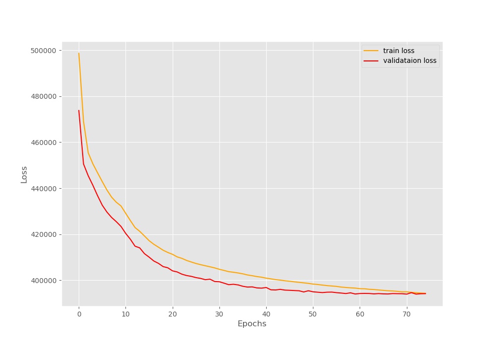
Figure 3. Loss plot after training the deep learning autoencoder model for 75 epochs.
We can see that the loss is starting at a pretty high value of around 500000. Does that mean that our model is not learning? Well, it is clearly visible that the loss is decreasing till the end of 75 epochs. This means that our model has learned at least something. But do take a careful look. At the end of 75 epoch, the train and validation loss lines are completely touching each other. So, any more training than this will result in overfitting of the model. Let’s park this discussion here. We will get to this part just a bit later.
Analyzing the Reconstructed Images
But we will get the best idea of how well our model has learned by taking a look at the reconstructed images. Has our model really learned to generate fictional celebrity faces? Maybe a few output images will clear that up.
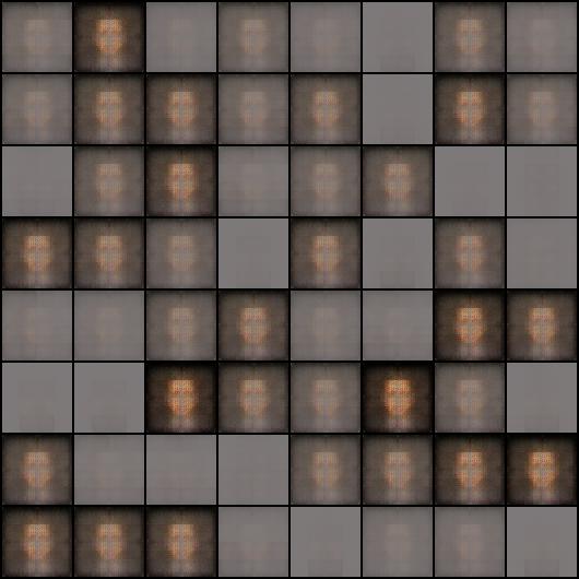
Figure 4. The image reconstructions by the convolutional variational autoencoder neural network after training for 1 epoch. Most of it just random noise with just a few formations of face like images.
Figure 4 shows the output after the first epoch. We can see that mostly it is noise and a figure which somewhat looks like a face. Certainly not a celebrity.
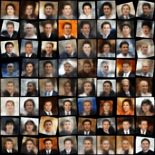
Now, taking a look at the output image after complete training, that is 75 epochs.
Figure 5. After 75 epochs, our autoencoder neural network is giving really good results. It is able to generate new faces with much more details now. It is even generating details like eyebrows and differentiating between the background and clothes of the people.
Now we have something. These images certainly look like human faces, if not celebrities. The images are pretty low resolution, still we can clearly see that the model has learned how to generate some important features like eyebrows, lips, and eyes. If you observe closely, then you can see that it in some cases the autoencoder neural network has learned to differentiate between the background color and the clothes of the persons.
Further, to get a complete idea of how the model is generating the images through the epochs, let’s have a look at the GIF file that we saved.
Clip 1. The output images that are generated by the convolutional variational autoencoder deep learning model through the epochs. We can see the different features and details is the neural network is learning throughout is training.
It is quite fascinating to see the deep learning autoencoder neural network learn through the epochs. Starting from random noise, slowly it learns to generate the colors, then the faces, and the intricate details of the faces as well. We can say that the model is performing quite in line with our expectations.
Further Experimentations with Convolutional Variational Autoencoder with PyTorch
If you wish to take this project further and learn even more about convolutional variational autoencoder using PyTorch, then you may consider the following steps.
You may consider using the original 250×250 dimensional images for training. Although you may have to change the model architecture a bit for that. That will also take longer to train and require more GPU memory as well.
Training any longer with the current learning rate values and planning will lead to overfitting. You can use a learning rate scheduler to train for longer or stop the training when the loss plateaus.
You can also apply the same model on a completely new dataset and observe how the model learns.
If you carry any of the above steps, you can share your findings in the comment section. This will surely help the other readers learn or even motivate them to do their own experiments.
Summary and Conclusion
In this article, you learned how to generate fictional celebrity faces using an autoencoder deep learning neural network. In particular, you used a convolutional variational autoencoder neural network along with the PyTorch deep learning library.
If you have any doubts, thoughts, or suggestions, then please share them in the comment section. I will surely address them.
You can contact me using the Contact section. You can also find me on LinkedIn, and X.
Liked it? Take a second to support Sovit Ranjan Rath on Patreon!
Hello Raj. Sorry to hear that you ran into those errors. Just one clarification from your side. Can you please double-check the folder structure and the directory from where you are executing the Python file. There might be some simple errors regarding those. If you face these errors still, then I will double-check the code from my side.
Thank you for writing such a wonderful blog. I must say this is very helpful for getting the implementational understanding of the VAE. However, I have one small confusion regarding the loss. I see it to be a combination of the KL divergence and BCE but it’s not normalized based on the number of samples in a batch. Could you help me with this, if it’s something you missed or is it a general practice. I feel it should have been normalized based on the number of samples in a batch. Please let me know your thoughts.
Hello.
Thank you for your appreciation.
I think what you are looking for is dividing the complete loss by the number of batches at the end of each epoch. If that’s what you are asking about, then we are doing that at the end of train() and validate() functions just before the return statement.
I hope that this clarifies your doubt.
I see what you mean but that’s not what I meant. The reason why I wanted to check for the normalization of loss for each batch with respect to the number of samples is: I have many examples in the train set but very few in the val set. My train set has approx 2k records but val set has approx 100. So if my batch size is 256 then the val and train loss is in different magnitudes cause for train set I have many complete (batch having 256 examples) batch but not even a single “complete” batch for val set. So the ideal solution I thought was to normalize the loss for each batch based on the number of records in each batch. Let me know if this is making sense.
I see what you mean. Instead of normalizing after each epoch (as it is in the current post), you want to normalize after each batch. I will give it a thought and if possible try to run the training. But if you have already ran the training, can you please let me know about your findings.
I did train a model but it was for a different dataset (chest x-ray images). What I found was if I directly use your code then train loss (after one epoch) was around 20k and val loss (after one epoch – with only one incomplete batch) was around 2k.
Here is what I changed for both the train and val loss calculation.
running_loss += (loss.item()/len(data))
Now my train and val loss are nearly similar (which should be expected imo)
Hello. I am starting a new thread here as the previous one won’t allow any more. But that may be a bit wrong. In your case you are dividing the current batch loss by total samples in the dataset. Instead try running_loss += (loss.item()/dataloader.batch_size)
This website uses cookies so that we can provide you with the best user experience possible. Cookie information is stored in your browser and performs functions such as recognising you when you return to our website and helping our team to understand which sections of the website you find most interesting and useful.
Strictly Necessary Cookies
Strictly Necessary Cookie should be enabled at all times so that we can save your preferences for cookie settings.
If you disable this cookie, we will not be able to save your preferences. This means that every time you visit this website you will need to enable or disable cookies again.


Getting error
import model
(Error as No module named ‘model’)
And
From engine import train,validate
(Error as no module name ‘engine’)
Hello Raj. Sorry to hear that you ran into those errors. Just one clarification from your side. Can you please double-check the folder structure and the directory from where you are executing the Python file. There might be some simple errors regarding those. If you face these errors still, then I will double-check the code from my side.
Hi Sovit,
Thank you for writing such a wonderful blog. I must say this is very helpful for getting the implementational understanding of the VAE. However, I have one small confusion regarding the loss. I see it to be a combination of the KL divergence and BCE but it’s not normalized based on the number of samples in a batch. Could you help me with this, if it’s something you missed or is it a general practice. I feel it should have been normalized based on the number of samples in a batch. Please let me know your thoughts.
Hello.
Thank you for your appreciation.
I think what you are looking for is dividing the complete loss by the number of batches at the end of each epoch. If that’s what you are asking about, then we are doing that at the end of train() and validate() functions just before the return statement.
I hope that this clarifies your doubt.
I see what you mean but that’s not what I meant. The reason why I wanted to check for the normalization of loss for each batch with respect to the number of samples is: I have many examples in the train set but very few in the val set. My train set has approx 2k records but val set has approx 100. So if my batch size is 256 then the val and train loss is in different magnitudes cause for train set I have many complete (batch having 256 examples) batch but not even a single “complete” batch for val set. So the ideal solution I thought was to normalize the loss for each batch based on the number of records in each batch. Let me know if this is making sense.
I see what you mean. Instead of normalizing after each epoch (as it is in the current post), you want to normalize after each batch. I will give it a thought and if possible try to run the training. But if you have already ran the training, can you please let me know about your findings.
I did train a model but it was for a different dataset (chest x-ray images). What I found was if I directly use your code then train loss (after one epoch) was around 20k and val loss (after one epoch – with only one incomplete batch) was around 2k.
Here is what I changed for both the train and val loss calculation.
running_loss += (loss.item()/len(data))
Now my train and val loss are nearly similar (which should be expected imo)
Hello. I am starting a new thread here as the previous one won’t allow any more. But that may be a bit wrong. In your case you are dividing the current batch loss by total samples in the dataset. Instead try running_loss += (loss.item()/dataloader.batch_size)