Autoencoder Neural Network: Application to Image Denoising

Updated: March 25, 2020.

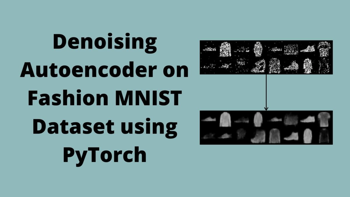
One of the applications of deep learning autoencoders is image reconstruction. But it is not necessary that the input images will always be clean. Sometimes, the input images for autoencoders can be noisy. In that case, the deep learning autoencoder has to denoise the input images, get the hidden code representation, and then reconstruct the original images. It is one of the useful applications of autoencoders in deep learning.

In this article, we will be learning about denoising autoencoders, how they work, and how to implement them using PyTorch machine learning library.

• What Will We Cover in this Article?
  • – A brief introduction to denoising autoencoders.
  • – Adding noise to images.
  • – Coding our denoising convolutional autoencoder in PyTorch.
  • – Analyzing the plots, images, and results.

• If you want to get some more knowledge on autoencoder before moving further, then consider reading my previous article:
  • Autoencoders in Deep Learning.
  • Implementing Deep Autoencoder in PyTorch.
  • Machine Learning Hands-On: Convolutional Autoencoders.

Introduction to Denoising Autoencoders

Denoising autoencoders are an extension of the basic autoencoders architecture. An autoencoder neural network tries to reconstruct images from hidden code space. In denoising autoencoders, we will introduce some noise to the images. The denoising autoencoder network will also try to reconstruct the images. But before that, it will have to cancel out the noise from the input image data. In doing so, the autoencoder network will learn to capture all the important features of the data.

Loss Function for Denoising Autoencoder Networks

Training a denoising autoencoder results in a more robust neural network model that can handle noisy data quite well.

In a regular autoencoder network, we define the loss function as,

$$
L(x, r) = L(x, \ g(f(x)))
$$

where \(L\) is the loss function, \(x\) is the input, and \(r \ = \ g(f(x))\) is the reconstruction by the decoder. In this case, the loss function can be squared error.

Now, when we take the case of denoising autoencoders, then we tend to add some noise to the input data \(x\) to make it \(\tilde{x}\). Here, the loss function becomes the following.

$$
L(x, r) = L(x, \ g(f(\tilde{x})))
$$

In the above, loss function, \(\tilde{x}\) is the noisy data, and the reconstruction \(r \ = \ g(f(\tilde{x}))\).

In the autoencoder network, the loss function always introduces a penalty when the input \(x\) is dissimilar from the reconstruction \(r\). (Deep Learning by Ian Goodfellow, Yoshua Bengio and Aaron Courville, Autoencoders Chapter, page 500).

If the loss function is the squared error loss, then we can make it a bit more specific with the following equation.

$$
l = \frac{1}{2} \sum_{i=1}^N (x_{i} – \hat{\tilde{x_{i}}})^2
$$

where \(N\) is the total number of training examples.

In practical coding, we generally take the MSELoss (Mean Squared Error) for training the autoencoder deep neural network. We will be learning more about it once we start the code part of this article.

Okay, I hope that the above theory makes the concepts clearer.

Adding Noise to Images

We will need noisy images for the inputs, and for that, we will be adding noise manually to the images.

In this article, we will use the Fashion MNIST image dataset.

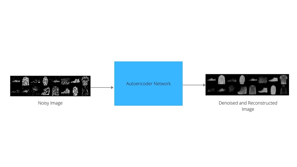
So, all in all, we will give noisy images as inputs to the autoencoder neural network, then the encoder neural network will try to get the compress latent space representation. And the decoder part of the network will reconstruct the images. We will finally get to see how well our model performs after training when we give test images for denoising and reconstruction to it.

Moving to the coding part of the article now.

If you have been following my previous articles, or have gone through those before reading this, then you may find that the main changes in the code part take place in the neural network model, the train function and the test function.

Importing Modules and Libraries

Let’s import all the modules that we will need.

# imports
import os
import torch 
import torchvision
import numpy as np
import torch.nn as nn
import torchvision.transforms as transforms
import torch.optim as optim
import matplotlib.pyplot as plt
import torch.nn.functional as F

from torchvision import datasets
from torch.utils.data import DataLoader
from torchvision.utils import save_image

• You must be familiar with most the above imports, still I am including the description for a few important ones.
  • torchvision: contains many popular computer vision datasets, deep neural network architectures, and image processing modules. We will use this to download the Fashion MNIST dataset.
  • torch.nn: contains the deep learning neural network layers such as Linear(), and Conv2d().
  • transforms: will help in defining the image transforms and normalizations.
  • optim: contains the deep learning optimizer classes such as MSELoss() and many others as well.
  • functional: we will use this for activation functions such as ReLU.
  • DataLoader: eases the task of making iterable training and testing sets.
  • save_image: torchvision.utils provides this module to easily save PyTorch tensor images.

Define Constants

Here, we will define some constants that will become helpful along the way later in the code.

# constants
NUM_EPOCHS = 10
LEARNING_RATE = 1e-3
BATCH_SIZE = 16
NOISE_FACTOR = 0.5

So, we will train our model for 10 epochs, with a learning rate of 0.001, and a batch size of 16. If you have more memory at your disposal, then maybe you can increase the batch size to 32 or 64. We also have the constant NOISE_FACTOR which defines the amount of noise that we will add to our images. It will become clearer further along the way when we will actually add noise to the images.

Prepare the Data

We can now define our image transforms, and prepare our training and test set as well.

First, let’s define the transforms for our images.

# transforms
transform = transforms.Compose([
    transforms.ToTensor(),
    transforms.Normalize((0.5,), (0.5,)),
])

In the above code block, we are converting the image pixel data to PyTorch tensors, and normalizing the values as well (lines 2 – 5). Normalizing the pixel values will lead them to be within the range [0, 1]. This ensures faster training than the default pixel value range, which is [0, 256].

The following code block prepares our trainloader and testloader set for training and testing respectively.

trainset = datasets.FashionMNIST(
    root='./data',
    train=True, 
    download=True,
    transform=transform
)
testset = datasets.FashionMNIST(
    root='./data',
    train=False,
    download=True,
    transform=transform
)

trainloader = DataLoader(
    trainset, 
    batch_size=BATCH_SIZE,
    shuffle=True
)
testloader = DataLoader(
    testset, 
    batch_size=BATCH_SIZE, 
    shuffle=True
)

Some Helper Functions

Next, we have some helper functions that will make our work easier along the way. The following are those functions.

def get_device():
    if torch.cuda.is_available():
        device = 'cuda:0'
    else:
        device = 'cpu'
    return device
def make_dir():
    image_dir = 'Saved_Images'
    if not os.path.exists(image_dir):
        os.makedirs(image_dir)
def save_decoded_image(img, name):
    img = img.view(img.size(0), 1, 28, 28)
    save_image(img, name)

The first function is get_device() (lines 1 – 6), which either returns the CUDA GPU device or the CPU depending upon the availability. This is better than writing manual code as we just need to call this function and get the computation device automatically.

The next one is the make_dir() (line 7 – 10) function which makes a directory called Saved_Image. This directory saves noisy images and the corresponding denoised images while training the autoencoder neural network. This is not really required as a function. You can write it as a direct code also.

The last function is save_decoded_image() (lines 11 – 13). This function takes two arguments. One is the image tensor, and the other one is the path of the image as a string. This saves the images in the Saved_Images directory.

Define the Autoencoder Neural Network

The next step is to define our Autoencoder class. First, we will define all our layers required in the __init__() function. Then we will build our deep neural network in the forward() function. Let’s write the code, then we will get to the explanation part.

# the autoencoder network
class Autoencoder(nn.Module):
    def __init__(self):
        super(Autoencoder, self).__init__()

        # encoder layers
        self.enc1 = nn.Conv2d(1, 64, kernel_size=3, padding=1)
        self.enc2 = nn.Conv2d(64, 32, kernel_size=3, padding=1)
        self.enc3 = nn.Conv2d(32, 16, kernel_size=3, padding=1)
        self.enc4 = nn.Conv2d(16, 8, kernel_size=3, padding=1)
        self.pool = nn.MaxPool2d(2, 2)
        
        # decoder layers
        self.dec1 = nn.ConvTranspose2d(8, 8, kernel_size=3, stride=2)  
        self.dec2 = nn.ConvTranspose2d(8, 16, kernel_size=3, stride=2)
        self.dec3 = nn.ConvTranspose2d(16, 32, kernel_size=2, stride=2)
        self.dec4 = nn.ConvTranspose2d(32, 64, kernel_size=2, stride=2)
        self.out = nn.Conv2d(64, 1, kernel_size=3, padding=1)


    def forward(self, x):
        # encode
        x = F.relu(self.enc1(x))
        x = self.pool(x)
        x = F.relu(self.enc2(x))
        x = self.pool(x)
        x = F.relu(self.enc3(x))
        x = self.pool(x)
        x = F.relu(self.enc4(x))
        x = self.pool(x) # the latent space representation
        
        # decode
        x = F.relu(self.dec1(x))
        x = F.relu(self.dec2(x))
        x = F.relu(self.dec3(x))
        x = F.relu(self.dec4(x))
        x = F.sigmoid(self.out(x))

        return x

net = Autoencoder()
print(net)

In the __init__() function (lines 3 to 18) we have defined all the layers that we will use while constructing the neural network model. First, we have the encoding layers which consist of nn.Conv2d() layers and one nn.MaxPool2d() layer. Starting from self.enc1, we have in_channels=1. The 1 represents that the image is grayscale having only a single color channel. We have out_channels=64, kernel_size=3, and padding=1. Then we keep on decreasing our out_channels till we have 8 in self.enc4. Then we have the nn.MaxPool2d() with both kernels and stride with value 2.

The decoding layers consist of nn.ConvTranspose2d(). Starting from self.dec1 we keep on increasing the dimensionality till we get 64 out_channels in self.dec4. Finally, there is an nn.Conv2d() layer with 1 output channel so as to reconstruct the original image.

In the forward() function, we stack up all our layers to perform encoding first. Each of the encoding layers is passed through the ReLU activation function. We also have the pooling layer after each convolutional layer. At line 30 we obtain the latent space code representation of the input data. The decoding of the latent space representation takes place from lines 33 to 37. Again all the ConvTranspose2d() go through the ReLU activation function. The final decoding layer is coupled with the sigmoid activation function. Finally, we return our network and instantiate a net object of the Autoencoder class.

Printing the neural network will give the following output.

Autoencoder(
  (enc1): Conv2d(1, 64, kernel_size=(3, 3), stride=(1, 1), padding=(1, 1))
  (enc2): Conv2d(64, 32, kernel_size=(3, 3), stride=(1, 1), padding=(1, 1))
  (enc3): Conv2d(32, 16, kernel_size=(3, 3), stride=(1, 1), padding=(1, 1))
  (enc4): Conv2d(16, 8, kernel_size=(3, 3), stride=(1, 1), padding=(1, 1))
  (pool): MaxPool2d(kernel_size=2, stride=2, padding=0, dilation=1, ceil_mode=False)
  (dec1): ConvTranspose2d(8, 8, kernel_size=(3, 3), stride=(2, 2))
  (dec2): ConvTranspose2d(8, 16, kernel_size=(3, 3), stride=(2, 2))
  (dec3): ConvTranspose2d(16, 32, kernel_size=(2, 2), stride=(2, 2))
  (dec4): ConvTranspose2d(32, 64, kernel_size=(2, 2), stride=(2, 2))
  (out): Conv2d(64, 1, kernel_size=(3, 3), stride=(1, 1), padding=(1, 1))
)

The Optimizer and Loss Function

Here, we will define the optimizer and loss for our neural network.

# the loss function
criterion = nn.MSELoss()
# the optimizer
optimizer = optim.Adam(net.parameters(), lr=LEARNING_RATE)

The loss function is MSELoss, and the optimizer is Adam optimizer. We are using mean squared error as the loss function as each of the values that the neural network predicts will be image pixel values which are numbers. Therefore, we need the mean squared error to calculate the dissimilarity between the original pixel values and the predicted pixel values.

Define the Training and the Test Function

We will manually add noise to the images batch-wise. First, we will add noise to the training images. Then, we will use those noisy images for training our network. The same goes for the testing phase as well. We will add noise to the test images, and give them to our autoencoder network in the hope that it will give us denoised images as output.

The following is the training function that we will be using.

# the training function
def train(net, trainloader, NUM_EPOCHS):
    train_loss = []
    for epoch in range(NUM_EPOCHS):
        running_loss = 0.0
        for data in trainloader:
            img, _ = data # we do not need the image labels
            # add noise to the image data
            img_noisy = img + NOISE_FACTOR * torch.randn(img.shape)
            # clip to make the values fall between 0 and 1
            img_noisy = np.clip(img_noisy, 0., 1.)
            img_noisy = img_noisy.to(device)
            optimizer.zero_grad()
            outputs = net(img_noisy)
            loss = criterion(outputs, img_noisy)
            # backpropagation
            loss.backward()
            # update the parameters
            optimizer.step()
            running_loss += loss.item()
        
        loss = running_loss / len(trainloader)
        train_loss.append(loss)
        print('Epoch {} of {}, Train Loss: {:.3f}'.format(
            epoch+1, NUM_EPOCHS, loss))

        save_decoded_image(img_noisy.cpu().data, name='./Saved_Images/noisy{}.png'.format(epoch))
        save_decoded_image(outputs.cpu().data, name='./Saved_Images/denoised{}.png'.format(epoch))

    return train_loss

The train function takes the net object, the trainloader and the number of epochs as the arguments. In the above code block, we add noise to the images (line 9) according to our NOISE_FACTOR constant that we have defined earlier in this article. One important point here is that we clip the values of the noisy images as well (line 11). This ensures that the pixel values are still within the range [0, 1]. We then load the noisy images on to the computation device, get the loss values, backpropagate the gradients. Then we update the parameters with optimizer.step() and add the losses to running_loss variable. You should always remember to perform optimizer.zero_grad() for each batch so as to make the gradients zero at the beginning of the batch. After each epoch, we are printing the training loss and saving the images as well.

Next, getting to the test function.

def test_image_reconstruction(net, testloader):
     for batch in testloader:
        img, _ = batch
        img_noisy = img + NOISE_FACTOR * torch.randn(img.shape)
        img_noisy = np.clip(img_noisy, 0., 1.)
        img_noisy = img_noisy.to(device)
        outputs = net(img_noisy)
        outputs = outputs.view(outputs.size(0), 1, 28, 28).cpu().data
        save_image(img_noisy, 'noisy_test_input.png')
        save_image(outputs, 'denoised_test_reconstruction.png')
        break

During testing, we add noise to the images and clip the values as well (lines 4 and 5). But here, we do not backpropagate the gradients and perform the image reconstruction for only one batch. You can perform image reconstruction for the entire test set if you want.

Everything is set up now, and we just have to call the functions that we have defined. So, let’s do that now.

device = get_device()
print(device)
net.to(device)
make_dir()
train_loss = train(net, trainloader, NUM_EPOCHS)
plt.figure()
plt.plot(train_loss)
plt.title('Train Loss')
plt.xlabel('Epochs')
plt.ylabel('Loss')
plt.savefig('./Saved_Images/conv_ae_fahsionmnist_loss.png')
test_image_reconstruction(net, testloader)

Train Loss Plot

The following lines show the loss values while training.

Epoch 1 of 10, Train Loss: 0.062
Epoch 2 of 10, Train Loss: 0.057
Epoch 3 of 10, Train Loss: 0.056
Epoch 4 of 10, Train Loss: 0.055
Epoch 5 of 10, Train Loss: 0.055
Epoch 6 of 10, Train Loss: 0.055
Epoch 7 of 10, Train Loss: 0.055
Epoch 8 of 10, Train Loss: 0.055
Epoch 9 of 10, Train Loss: 0.055
Epoch 10 of 10, Train Loss: 0.055

We can see that the loss values do not decrease after 4 epochs. Maybe a bigger network will be able to perform better. Taking a look at the loss plot.

Obviously training a bigger network and training for more epochs will yield better results. You can also play with the learning rate to analyze the changes. Now, let’s take a look at the test image reconstruction that our autoencoder network has performed.

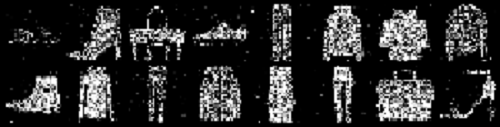
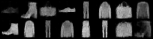
The first image shows the noisy image that we have given as input to our neural network. And the second image shows the denoised and reconstructed image. The model performs well, but still, the image comes out a bit blurry.

Summary and Conclusion

I hope that you learned a lot from this article, and are ready to carry our further experimentations on your own. If you want to know more about autoencoders in general, then you may like the following resources.

• More resources on autoencoders
  • Deep Learning by Ian Goodfellow, Yoshua Bengio and Aaron Courville, Autoencoders Chapter, page 500.
  • Research paper – Stacked denoising autoencoders: Learning useful representations in a deep network with a local denoising criterion, Pascal Vincent, Hugo Larochelle, Isabelle Lajoie, Yoshua Bengio, Pierre-Antoine Manzagol.
  • Research paper – Autoencoders, Minimum Description Length, and Helmholtz Free Energy, Geoffrey E. Hinton, Richard S. Zemel.

Feel free to ask questions and point out any inconsistencies in the article in the comment section. I will try my best to address them. You can find me on LinkedIn, and Twitter as well.