
Autoencoder deep neural networks are an unsupervised learning technique. Autoencoders are really good at mapping the input to the output. The output is mostly a compressed representation of the input data. And in the process of copying the input data to the output data, they learn many features about the data. In this article, we will learn about sparse autoencoders. Specifically, we will cover the following about sparse autoencoders in this article:
- A brief about deep autoencoder.
- Problems with deep autoencoders.
- What are sparse autoencoders?
- Why are sparse autoencoders important?
- How to code a sparse autoencoder using PyTorch deep learning library?
In a series of previous articles, I have described the working of autoencoders, deep autoencoders, convolutional autoencoders, and denoising autoencoders. The following are those articles:
- Autoencoders in Deep Learning.
- Implementing Deep Autoencoder in PyTorch.
- Machine Learning Hands-On: Convolutional Autoencoders.
- Autoencoder Neural Network: Application to Image Denoising.
- Denoising Text Image Documents using Autoencoders.
You can refer to the above articles if you are starting out with autoencoder neural networks. I hope that you will learn a lot, and I will love to know your thoughts in the comment section.
A Brief About Autoencoders
Basically, autoencoding is a data compressing technique. An autoencoder has two parts, the encoder, and the decoder. The autoencoder neural network learns to recreate a compressed representation of the input data.
The encoder encodes the data, and the decoder decodes the data. For example, let the input data be \(x\). Then, we can define the encoding function as \(f(x)\). A hidden layer \(h\) learns the encoding and we get, \(h = f(x)\). Finally, a decoding function \(g\) reconstructs the input as \(r = g(h)\). You can learn more about the basics of autoencoders from this article.
Problems with Deep Autoencoder
We know that autoencoders in general, try to map the input data to the output data.
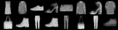
Take the case of a deep fully connected neural network autoencoder. Suppose that, you are trying to map the very popular FashionMNIST images. And you give the number of input neurons the same as the number of pixels, that is 784. In such cases, there is a very high probability that the autoencoder neural network autoencoder will just copy the input as it is after a few epochs of training. It will not able to learn any important features of the data. The following image will give you a better idea.
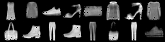
FashionMNIST reconstructed image by autoencoder without any sparsity.
The above image shows FashionMNIST reconstructed image by autoencoder without adding any sparsity. We can see that the model is reaching a point where it will be remember everything about the images and just copy them. Maybe a few more iterations and it will be able to do that. We want to avoid this.
Why are Sparse Autoencoders Important?
Now moving on to sparse autoencoders. In sparse autoencoders, we can still use fully connected neurons with numbers equal to the image dimensionality. But still, by adding a sparsity regularization, we will be able to stop the neural network from copying the input.
Mainly, there are two ways to add sparsity constraints to deep autoencoders.
- L1 regularization, which we will use in this article.
- KL divergence, which we will address in the next article.
How to Use L1 Regularization for Sparsity
We will add the L1 sparsity constraint to the activations of the neuron after the ReLU function. This will make some of the weights to be zero which will add a sparsity effect to the weights.
The following formula will make things clearer.
$$
L1 = \lambda * \sum|w_{i}|
$$
Here, \(\lambda\) is the regularization parameter, and \(w_{i}\)s are the activation weights. We will add this regularization to the loss function, say MSELoss. So, the final cost will become,
$$
Cost = MSELoss + \lambda * \sum|w_{i}|
$$
We will implement all of this through coding, and then, things will become even clearer.
Sparse Autoencoders Neural Network using PyTorch
We will use the FashionMNIST dataset for this article. Along with that, PyTorch deep learning library will help us control many of the underlying factors. We can experiment our way through this with ease.
Before moving further, I would like to bring to the attention of the readers this GitHub repository by tmac1997. It has an implementation of the L1 regularization with autoencoders in PyTorch. We will be using some of the code. Although we will need to change the code for our particular use case.
Let’s start with the coding.
Directory Structure
For this tutorial, we will use the following directory structure.
├───input
├───outputs
│   └───images
└───src
        sparse_ae_l1.py
inputfolder will contain the FashionMNIST images that we will download using thetorchvisiondatasetsmodule.outputswill contain the trained model that we will save and the loss plot as well. The subdirectoryimageswill contain the images that the autoencoder will reconstruct on the validation dataset.srccontains the python filesparse_ae_l1.py, that will contain all of the python code that we will write.
Importing Modules
import torch
import torchvision
import torch.nn as nn
import matplotlib
import matplotlib.pyplot as plt
import torchvision.transforms as transforms
import torch.nn.functional as F
import torch.optim as optim
import os
import time
import numpy as np
import argparse

from tqdm import tqdm
from torchvision import datasets
from torch.utils.data import DataLoader
from torchvision.utils import save_image

matplotlib.style.use('ggplot')
Some of the important modules that we are using are:
torchvisionto get the FashionMNIST dataset, apply transforms, and save the torch tensors easily as images.torch.nnfor accessing the neural network layers and activations in PyTorch.DataLoaderto prepare the iterable data loader to feed into the neural network model.argparseto construct the argument parser.
Constructing the Argument Parsers
We will now construct the argument parser. Using command line arguments while executing the python file will make it easier for us to control some important parameters.
# constructing argument parsers
ap = argparse.ArgumentParser()
ap.add_argument('-e', '--epochs', type=int, default=10,
	help='number of epochs to train our network for')
ap.add_argument('-l', '--reg_param', type=float, default=0.001,
    help='regularization parameter `lambda`')
ap.add_argument('-sc', '--add_sparse', type=str, default='yes',
    help='whether to add sparsity contraint or not')
args = vars(ap.parse_args())

epochs = args['epochs']
reg_param = args['reg_param']
add_sparsity = args['add_sparse']
learning_rate = 1e-3
batch_size = 32

print(f"Add sparsity regularization: {add_sparsity}")
--epochsdefines the number of epochs that we will train our autoencoder neural network for.--reg_paramis the regularization parameter lambda.--add_sparseis a string, either ‘yes’ or ‘no’. It tells whether we want to add the L1 regularization constraint or not. And obviously, it will be ‘yes’ in this tutorial.- On lines 11, 12, and 13 we are initializing the arguments as well, so that they will be easier to use further along.
- On lines 14 and 15 we are specifying the learning rate and batch size.
Prepare the Data
We will download the dataset using the torchvision dataset module. We will also apply transforms to the image data. For the transforms, we will only convert the data into torch tensors.
# image transformations
transform = transforms.Compose([
    transforms.ToTensor(),
])

trainset = datasets.FashionMNIST(
    root='../input/data',
    train=True,
    download=True,
    transform=transform
)
testset = datasets.FashionMNIST(
    root='../input/data',
    train=False,
    download=True,
    transform=transform
)

# trainloader
trainloader = DataLoader(
    trainset,
    batch_size=batch_size,
    shuffle=True
)
#testloader
testloader = DataLoader(
    testset,
    batch_size=batch_size,
    shuffle=False
)
- First at line 2, we define the transforms.
- Then from lines 6 to 17, we download the training and test dataset that will be stored in
input/datafolder. If you already have the dataset, then it will not be downloaded. - From lines 19 to 30, we prepare the iterable train loader and test loader using PyTorch
DataLoader. The batch size is 32 and we are only shuffling the train loader.
Some Helper Functions
In this section, we will define some helper functions that will make our work a little bit easier and automated. So, we will define three functions, namely, get_device(), make_dir(), and save_decoded_image(). Let’s write the code first, then we will get into the explanation part.
# get the computation device
def get_device():
    if torch.cuda.is_available():
        device = 'cuda:0'
    else:
        device = 'cpu'
    return device
device = get_device()

# make the `images` directory
def make_dir():
    image_dir = '../outputs/images'
    if not os.path.exists(image_dir):
        os.makedirs(image_dir)
make_dir()

# for saving the reconstructed images
def save_decoded_image(img, name):
    img = img.view(img.size(0), 1, 28, 28)
    save_image(img, name)
- Starting from line 2, we define the
get_device()function. This will grab either the CUDA GPU device or the CPU for computational purposes during the training of the autoencoder neural network model. Although it is not necessary to have a GPU for working with the Fashion MNIST dataset, still it is always better to have one for neural network training purposes. - Next from line 11, we define
make_dir(). This function creates animagesfolder inside theoutputsfolder. Here, we will save all the images that are reconstructed by the autoencoder during validation. - Finally, from lines 18 to 20 we define
save_decoded_image(). This function will save all the torch tensor outputs as images by resizing them into 28x28x1 dimensionality. It takes two input parameters, the image tensors, and the name of the file.
This finishes all of the preliminary coding parts. Now, we can get into the neural network coding and the core of this article. That is, training an autoencoder neural network with the sparsity penalty.
Define the Sparse Autoencoder Neural Network
In this section, we will define our sparse autoencoder neural network module.
An autoencoder neural network will have two parts, an encoder, and a decoder. We will only use nn.Linear layers of PyTorch deep learning library. We will not be using convolutional layers.
Let’s name our module SparseAutoencoder(). The following code block defines the SparseAutoencoder() module.
# define the autoencoder model
class SparseAutoencoder(nn.Module):
    def __init__(self):
        super(SparseAutoencoder, self).__init__()

        # encoder
        self.enc1 = nn.Linear(in_features=784, out_features=256)
        self.enc2 = nn.Linear(in_features=256, out_features=128)
        self.enc3 = nn.Linear(in_features=128, out_features=64)
        self.enc4 = nn.Linear(in_features=64, out_features=32)
        self.enc5 = nn.Linear(in_features=32, out_features=16)

        # decoder
        self.dec1 = nn.Linear(in_features=16, out_features=32)
        self.dec2 = nn.Linear(in_features=32, out_features=64)
        self.dec3 = nn.Linear(in_features=64, out_features=128)
        self.dec4 = nn.Linear(in_features=128, out_features=256)
        self.dec5 = nn.Linear(in_features=256, out_features=784)

    def forward(self, x):
        # encoding
        x = F.relu(self.enc1(x))
        x = F.relu(self.enc2(x))
        x = F.relu(self.enc3(x))
        x = F.relu(self.enc4(x))
        x = F.relu(self.enc5(x))

        # decoding
        x = F.relu(self.dec1(x))
        x = F.relu(self.dec2(x))
        x = F.relu(self.dec3(x))
        x = F.relu(self.dec4(x))
        x = F.relu(self.dec5(x))
        return x
model = SparseAutoencoder().to(device)
- In
__init__(), starting from line 7, first, we have the encoder part of the autoencoder network. We have five encoder layers, starting from 784in_features. This refers to the 784 pixels that the Fashion MNIST images have. Continuing to reduce this untilself.enc5, we have 32in_featuresand 16out_features. - Then from lines 14 to 18, we define the decoder part of the network. Starting from
self.dec1tillself.dec5, we keep on increasing the number of neurons. This continues till we reach 784out_featuresinself.dec5. - We have the
forward()function from line 20. This executes the real encoding and decoding functionalities of our autoencoder neural network. All the encoder and decoder neural network layers go through ReLU activation functions when the encoding and decoding happens. - Next, we initialize the
SparseAutoencoder()module and load it onto the computation device.
We also need the loss function and optimizer for our autoencoder neural network model.
Loss Function and Optimizer
For the loss function, we will use MSELoss (Mean Squared Error Loss) as we need the error between the actual pixels and the reconstructed pixels. The optimizer is going to be Adam with a learning rate of 0.001.
# the loss function
criterion = nn.MSELoss()
# the optimizer
optimizer = optim.Adam(model.parameters(), lr=learning_rate)
Computing the Sparse Loss
To compute the sparse loss, we will need the activation weights of the neural network model. This means that the sparsity gets computed after the model parameters have passed through the ReLU activation functions. Only calculating the sparsity on the model parameters will not prove to be useful.
First, we need to get a hold on all the model children.
# get the layers as a list
model_children = list(model.children())
You can print all the children and you will the following output.
Linear(in_features=784, out_features=256, bias=True)
Linear(in_features=256, out_features=128, bias=True)
Linear(in_features=128, out_features=64, bias=True)
Linear(in_features=64, out_features=32, bias=True)
Linear(in_features=32, out_features=16, bias=True)
Linear(in_features=16, out_features=32, bias=True)
Linear(in_features=32, out_features=64, bias=True)
Linear(in_features=64, out_features=128, bias=True)
Linear(in_features=128, out_features=256, bias=True)
Linear(in_features=256, out_features=784, bias=True)
We will define a sparse_loss() function that takes the autoencoder model and the images as input parameters. Then we will calculate the sparsity loss after the images pass through the model parameters and the ReLU activation function.
The following code block shows how to do this.
# define the sparse loss function
def sparse_loss(autoencoder, images):
    loss = 0
    values = images
    for i in range(len(model_children)):
        values = F.relu((model_children[i](values)))
        loss += torch.mean(torch.abs(values))
    return loss
- Starting from line 5, we execute a
forloop. Inside thisforloop, we calculate thevaluesas the model image pixels pass through the ReLU activation (line 6). - At line 7, we get the
lossas the mean of all thevaluesthat are calculated in theforloop. - Finally, we return the
loss.
One important thing to note here is that this is not the sparsity penalty. We will get the final sparsity penalty after we multiply reg_param with this loss and add it with the MSELoss.
The Training and Validation Functions
Here, we will define our training and validation functions. We will call them fit() and validate() respectively.
The Training Function
# define the training function
def fit(model, dataloader, epoch):
    print('Training')
    model.train()
    running_loss = 0.0
    counter = 0
    for i, data in tqdm(enumerate(dataloader), total=int(len(trainset)/dataloader.batch_size)):
        counter += 1
        img, _ = data
        img = img.to(device)
        img = img.view(img.size(0), -1)
        optimizer.zero_grad()
        outputs = model(img)
        mse_loss = criterion(outputs, img)
        if add_sparsity == 'yes':
            l1_loss = sparse_loss(model, img)
            # add the sparsity penalty
            loss = mse_loss + reg_param * l1_loss
        else:
            loss = mse_loss
        loss.backward()
        optimizer.step()
        running_loss += loss.item()

    epoch_loss = running_loss / counter
    print(f"Train Loss: {loss:.3f}")

    # save the reconstructed images every 5 epochs
    if epoch % 5 == 0:
        save_decoded_image(outputs.cpu().data, f"../outputs/images/train{epoch}.png")
    return epoch_loss
- The
fit()function takes three parameters, the autoencoder model, the data loader (trainloader), and the current epoch number. running_lossat line 5, will help us calculate the batch-wise loss. Also, we will use thecounterto calculate the per epoch loss.- From line 7, we iterate through the data. We only get the images (
img) at line 9 as we do not need the labels for the autoencoder neural network. - At line 11, we are flattening the images as they will be passed into linear layers and not convolutional layers.
- Line 12 updates the gradients to zero and we get the output at line 13.
- At line 14, we get the
mse_loss. Then at line 16, we call thesparse_lossfunction and calculate the final sparsity constraint at line 18. In our case, line 20 does not execute. - Line 21 backpropagates the gradients, line 22 updates the model parameters, and line 23 calculates the batch loss.
- We calculate the
epoch_lossat line 25 and save the trained reconstructed images every 5 epochs (lines 29 and 30). - Line 31, returns the
epoch_loss.
The Validation Function
In the validation function:
- We don’t need to backpropagate the gradients.
- We don’t update the model parameters.
And everything will be within the with torch.no_grad() block. Everything else will be similar to the fit() function.
# define the validation function
def validate(model, dataloader, epoch):
    print('Validating')
    model.eval()
    running_loss = 0.0
    counter = 0
    with torch.no_grad():
        for i, data in tqdm(enumerate(dataloader), total=int(len(testset)/dataloader.batch_size)):
            counter += 1
            img, _ = data
            img = img.to(device)
            img = img.view(img.size(0), -1)
            outputs = model(img)
            loss = criterion(outputs, img)
            running_loss += loss.item()

    epoch_loss = running_loss / counter
    print(f"Val Loss: {loss:.3f}")

    # save the reconstructed images every 5 epochs
    if epoch % 5 == 0:
        outputs = outputs.view(outputs.size(0), 1, 28, 28).cpu().data
        save_image(outputs, f"../outputs/images/reconstruction{epoch}.png")
    return epoch_loss
Executing the Training and Validation Functions
We will train and validate our autoencoder network by binding everything within a for loop.
# train and validate the autoencoder neural network
train_loss = []
val_loss = []
start = time.time()
for epoch in range(epochs):
    print(f"Epoch {epoch+1} of {epochs}")
    train_epoch_loss = fit(model, trainloader, epoch)
    val_epoch_loss = validate(model, testloader, epoch)
    train_loss.append(train_epoch_loss)
    val_loss.append(val_epoch_loss)
end = time.time()

print(f"{(end-start)/60:.3} minutes")

# save the trained model
torch.save(model.state_dict(), f"../outputs/sparse_ae{epochs}.pth")
train_lossandval_losslists will store the per epoch training and validation loss values. We need the values to plot the loss graph in the end.- We then train and validate our model as per the number of epochs that will be specified in the command line arguments.
- At line 16 we save the trained model as a
.pthfile.
In the end, we just need to save the loss plot.
# loss plots
plt.figure(figsize=(10, 7))
plt.plot(train_loss, color='orange', label='train loss')
plt.plot(val_loss, color='red', label='validataion loss')
plt.xlabel('Epochs')
plt.ylabel('Loss')
plt.legend()
plt.savefig('../outputs/loss.png')
plt.show()
Executing the Python File
To execute the sparse_ae_l1.py file, you need to be inside the src folder. From there, type the following command in the terminal.
python sparse_ae_l1.py --epochs=25 --add_sparse=yes
We are training the autoencoder model for 25 epochs and adding the sparsity regularization as well. Here is a short snippet of the output that we get.
Add sparsity regularization: yes
Linear(in_features=784, out_features=256, bias=True)
Linear(in_features=256, out_features=128, bias=True)
Linear(in_features=128, out_features=64, bias=True)
Linear(in_features=64, out_features=32, bias=True)
Linear(in_features=32, out_features=16, bias=True)
Linear(in_features=16, out_features=32, bias=True)
Linear(in_features=32, out_features=64, bias=True)
Linear(in_features=64, out_features=128, bias=True)
Linear(in_features=128, out_features=256, bias=True)
Linear(in_features=256, out_features=784, bias=True)
Epoch 1 of 25
Training
100%|██████████████████████████████████████████████████████████████████████████████████████████████████| 1875/1875 [00:44<00:00, 42.09it/s]
Train Loss: 0.051
Validating
313it [00:01, 200.41it/s]
Val Loss: 0.057
...
Training
100%|██████████████████████████████████████████████████████████████████████████████████████████████████| 1875/1875 [00:45<00:00, 41.25it/s]
Train Loss: 0.027
Validating
313it [00:01, 197.38it/s]
Val Loss: 0.032
Epoch 25 of 25
Training
100%|██████████████████████████████████████████████████████████████████████████████████████████████████| 1875/1875 [00:45<00:00, 41.01it/s]
Train Loss: 0.025
Validating
313it [00:01, 176.61it/s]
Val Loss: 0.032
Analyzing the Results
From the loss values, we can infer that our model is learning well. Still, we should take a look at the loss plots that we have saved. Later, we will also analyze the images that the autoencoder neural network has reconstructed.
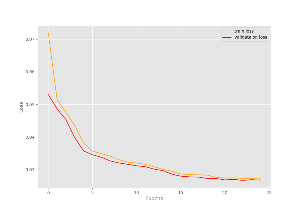
We can see that there is no overfitting while training the model which is a good thing. Now, taking a look at the reconstructed images by the autoencoder.
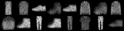
The first image shows the autoencoder reconstructed images after the first epoch. The images are blurry due to the additional sparsity penalty. After 20 epochs (the second image), the autoencoder is able to create somewhat clearer images. These images are still blurry but it is able to capture the important details like the handles of the bags.
These reconstructions are different from fully connected autoencoders without any sparsity. As in those cases, the autoencoder neural network can just copy the image if we train it long enough. But adding the sparsity penalty allows the autoencoder to capture the important details rather than just copying the input image to the output.
For gaining more knowledge about sparse autoencoders and regularization techniques you can read the following articles:
- Sparse autoencoder, Andrew Ng (CS294A Lecture notes).
- Differences between L1 and L2 as Loss Function and Regularization.
Summary and Conclusion
In this article, you learned how to add the L1 sparsity penalty to the autoencoder neural network so that it does not just copy the input image to the output. Rather it should be able to capture the important features of the images. In the next article, we will learn how to use KL-divergence for adding the sparsity penalty. If you have any thoughts, doubts, or suggestions, please leave them in the comment section. I will try my best to address them.
You can contact me using the Contact section. You can also find me on LinkedIn, and X.

Hello Sovit,
Thank you very much for your sharing! A little question, in the math part, the L1 regularization term is defined as the weighted sum of the absolute values of all the weights of neural network. However in the python code, it is calculated using the activations of each layer. I am wondering if I understand correctly? Are the two equivalent?
Thank you! Guangye
First of all, I am happy that you found the tutorial helpful. Now, coming to your question. Your question is quite good and relevant as well. For writing this article, I followed this paper by Andrew Ng https://web.stanford.edu/class/cs294a/sparseAutoencoder.pdf
Please do take look at PAGE 14. I am explaining my intuition here. After we apply activation to the units, then we only have those units’ weights which are active. No inactive unit’s weights are present. From the paper also I followed that it would make more sense to apply sparsity to those weights that are active only. We would not want to apply sparsity to all the weights and then discard them. This would mean some unnecessary operations would be discarded later. This is my take on it.
But if you have another thought on this, please do share. I would love to hear it.
Hello Sovit,
Thank you for your explanation! It’s very helpful.
Guangye
You are welcome and glad to help.
Hello
If we run this code on google colab, how can we access the images formed, also how will we be able to access the input and output folders?
Also, how to apply sparsity with convolutional autoencoders?
Hello AK. To run and access the images saved in Colab, we have to do a bit of folder setup in the Colab environment. Currently, I am trying to provide colab access for all my previous and future codes as well. That will take some time.
Now, coming to applying sparsity to convolutional autoencoders, I have not written an article on that till now. I will try my best to cover that in the future.
Hey I think your implementation of the flow for sparse loss only makes sense for if the loss is KL divergence, not L1 reg. L1 reg is the sum of abs of the values of weights (not the activation of linear layers’ outputs)
I will look it up. Not working with autoencoders that actively right now, so cannot say something concretely. Thanks for informing. If need be, I will update it.
I think sparsity should be applied to activations not weight. Isn’t it?
Hello. I will need to take a detailed look at the code. I wrote this article a long time ago and need to check again.
Still, thanks for bringing it to my attention.