Class Accuracies for Imbalanced Data in Deep Learning Image Recognition

In this article, we will discuss how to get per-class accuracy in a highly imbalanced image/vision dataset. Deep learning algorithms suffer when the dataset is highly imbalanced. In image recognition, a deep neural network may predict 90% of one class correctly and only 20% of another class correctly. This is the result of the number of images in each class when the dataset is imbalanced.

In the last article, I laid out a detailed approach on how to get above 95% accuracy on the Caltech101 dataset. I chose the problem as Caltech101 is a highly imbalanced vision dataset. But I only showed how to get the final accuracy on the test set.

I would suggest that you read the previous article before moving on with this article. This will help you to have a better grasp of what we are doing today.

Although we got 95% accuracy on the test set, we did not check the class-wise accuracy. Therefore, in this article, we will see how an imbalanced vision dataset affects class-wise accuracy. And obviously, we will deep neural networks in this article.

What Will We Cover in this Article?

• The dataset that we are going to use.
• The tools and libraries.
• The neural network model/architecture.
• Coding:
  • The directory structure.
  • Reading and preparing the data.
  • Dividing the data into training, validation, and test set.
  • Training our deep neural network model on the data.
  • Finding class-wise accuracy fog each category.
  • Averaging the accuracies to get a better glimpse at the results.

The Caltech256 Dataset

We will use the successor of the Caltech101 dataset, which is the Caltech256 dataset (Griffin, G. Holub, AD. Perona, P.The Caltech 256.).

The Caltech256 dataset has 30698 images in total spanning over 257 categories when including the clutter category. The clutter category has 827 images. But we will discard the clutter category and that will leave us with 256 categories for our use case.

Category Distribution in Caltech256 Vision Dataset

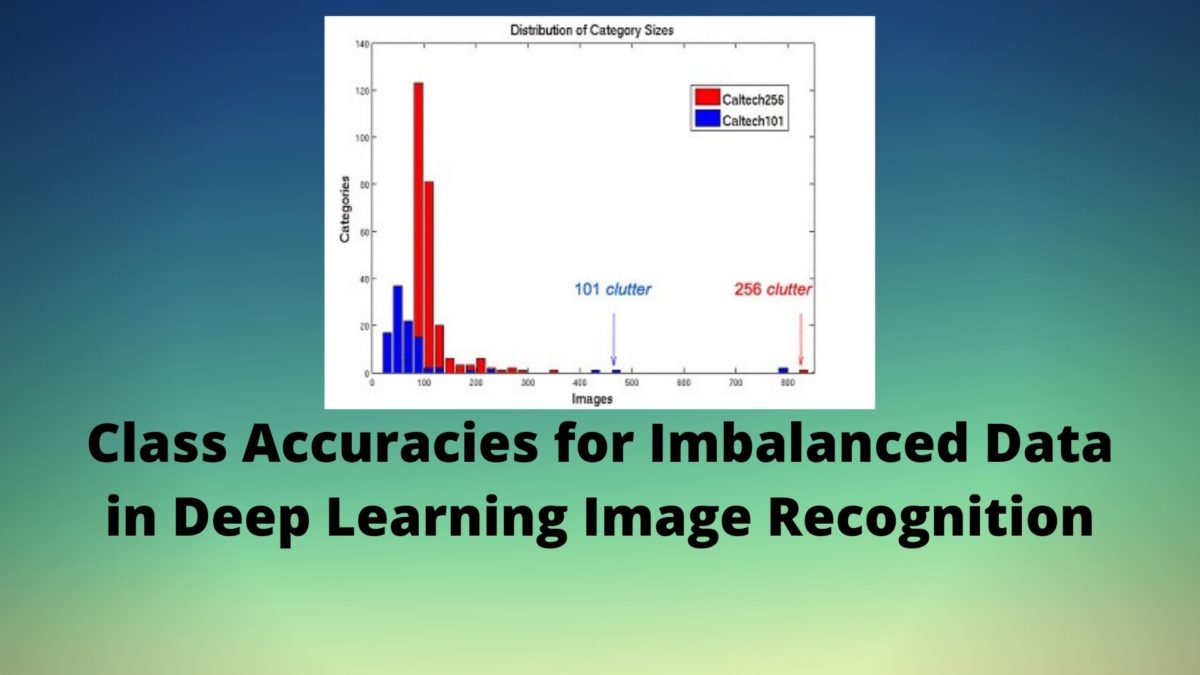
Actually how imbalanced is the Caltech256 vision dataset? The following bar plot will give a better idea of the image number distributions.

We can see that most of the categories have images between 80 and 150. Some of the categories have between 200 and 300 images. And clutter is the only category in the Caltech256 dataset with above 800 images (827 to be precise). Be sure to check out this slide show by the authors to have a better idea about the vision dataset.

Now, to get a better idea about the total distribution of images in the dataset, let’s take look at the following plot.

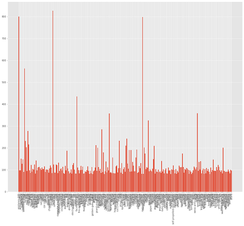
Although the labels are not visible due to so many classes, still this gives us a better idea about the distribution. Only two categories have above 800 images and clutter has 827 images. From the above plot, it is clearly visible that most of the categories have images between 80 and 150.

Also, the following are some of the classes along with the total number of images in those classes.

airplanes-101: 800
ak47: 98
american-flag: 97
backpack: 151
baseball-bat: 127
baseball-glove: 148
basketball-hoop: 90
...
welding-mask: 90
wheelbarrow: 91
windmill: 91
wine-bottle: 101
xylophone: 92
yarmulke: 84
yo-yo: 100
zebra: 96

Such imbalanced distribution can greatly affect the performance of neural networks in deep learning and image recognition.

Finding the final accuracy on a test set will not give us a good idea of how a deep neural network model performs on such imbalanced vision datasets. Therefore, in this article, we will find the per-class accuracy on the test set after training and validating our network.

Download the Caltech256 Vision Dataset

You will need the Caltech256 dataset further along. You can download the dataset from the official website.

After downloading the file, it will have a name 256_ObjectCategories.tar. Extract the contents and you will have a folder named 256_ObjectCategories. Inside this folder, there will be subdirectories. The name of these subdirectories are the categories and they contain all the images.

If you have followed my previous article, then you will know that this is very similar to the Caltech101 data.

The Directory Structure for This Tutorial

We are going to use the following directory structure for this article:

├───input
│   └───256_ObjectCategories
│       ├───001.ak47
│       ├───002.american-flag
│       ├───003.backpack
│       ├───004.baseball-bat
│       ├───005.baseball-glove
│       ├───006.basketball-hoop
...
├───outputs
└───src
    │   train.py

We have three directories, input, outputs, and src. input contains the 256_ObjectCategories folder which in turn contains the subdirectories along with the images. outputs will contain our trained model and accuracy and loss plots. And src contains the train.py file which is the python code file that we will edit.

Next, let’s move on to some of the major tools and libraries that we will be using.

Tools and Libraries

There are three important libraries/tools that you need to install to move further into the article. Those are imutils, PyTorch, and pretrained models. Please do install them before moving further.

• PyTorch.
• pretraindemodels:
  • pip install pretrainedmodels
• imutils:
  • pip install imutils

The Neural Network Architecture/Model that We Will Use

We will train a ResNet50 neural network model on the Caltech256 vision dataset. pretrainedmodels provides several types of pre-trained deep neural network models. These models are pre-trained on the ImageNet dataset. Be sure to check this amazing GitHub repository of computer vision pre-trained models.

For the ResNet50 neural network model, we will use the pre-trained ImageNet weights and fine-tune the head of the model, which is the classification layer of the neural network model.

Finding the Class Accuracies for Caltech256 Vision Dataset

Beginning from this section, we will get into the coding part of this tutorial.

Importing Libraries and Modules

We will start with all the required imports of the libraries and modules.

From here, you can put all of the code inside train.py python file. We will also set a seed so as to make our code reproducible across multiple runs.

import matplotlib.pyplot as plt
import matplotlib
import joblib
import cv2
import os
import torch 
import numpy as np
import torch.nn as nn
import torch.nn.functional as F
import torch.optim as optim
import time
import random
import pretrainedmodels

matplotlib.style.use('ggplot')

from imutils import paths
from sklearn.preprocessing import LabelBinarizer
from sklearn.model_selection import train_test_split
from torchvision.transforms import transforms
from torch.utils.data import DataLoader, Dataset
from tqdm import tqdm

'''
SEED Everything
'''
def seed_everything(SEED=42):
    random.seed(SEED)
    np.random.seed(SEED)
    torch.manual_seed(SEED)
    torch.cuda.manual_seed(SEED)
    torch.cuda.manual_seed_all(SEED)
    torch.backends.cudnn.benchmark = True # as we will resize the images
SEED=42
seed_everything(SEED=SEED)
'''
SEED Everything
'''

In the above code block, some of the important modules are:

• torch.nn will help us access the neural network layers in the PyTorch library.
• torch.optim to access all the optimizer functions in PyTorch.
• pretrainedmodels to access all the pre-trained models like ResNet34 and many more. We installed this library in one of the previous sections.
• Using torchvision.transforms we can apply transforms to our image like normalization and resizing.
• DataLoader and Dataset from the torchvision.transforms will help us to create our own custom image dataset module and iterable data loaders.
• cv2 to read images in the dataset.

Then starting from lines 27 to 35 we apply different seeds for the reproducibility of the results. One of the important ones among these is the torch.backends.cudnn.benchmark. We can keep this True as we will be resizing all the images to 224×224 pixels.

Setting the Computation Device

The following code block will choose the computation device for us, whether be it CUDA GPU or the CPU. Although I would recommend that you run the training on a GPU only as a CPU will be too inefficient and time-consuming.

# select the computation devie
if torch.cuda.is_available():
    device = 'cuda'
else:
    device = 'cpu'

epochs = 10

At line 7 we are setting the epoch as well.

Define the Transforms

Let’s define the image transforms that we will apply to the images. We will use torchvision.transforms to apply the transforms.

# define transforms
train_transform = transforms.Compose(
    [transforms.ToPILImage(),
     transforms.Resize((224, 224)),
     transforms.ToTensor(),
     transforms.Normalize(mean=[0.485, 0.456, 0.406],
                          std=[0.229, 0.224, 0.225])])
val_transform = transforms.Compose(
    [transforms.ToPILImage(),
     transforms.Resize((224, 224)),
     transforms.ToTensor(),
     transforms.Normalize(mean=[0.485, 0.456, 0.406],
                          std=[0.229, 0.224, 0.225])])

For the training set, we are defining train_transform (line 2). After resizing the images to 224×224, we are converting the images to tensors and normalizing the values as well. Note that we are not applying any image augmentation to the data.

Starting from line 10, we define val_transform for the validation set. We do not apply any augmentation to the validation set as well. Converting to tensors, resizing, and normalization of the pixel values are the only operations that we do on the validation set.

Get the Images and the Labels

Here, we will get the labels and the images as well. We will extract the label names from the name of the subdirectories which contain the images.

# get the paths
image_paths = list(paths.list_images('../input/256_ObjectCategories'))

data = []
labels = []
for image_path in tqdm(image_paths, total=len(image_paths)):
    label = image_path.split(os.path.sep)[-2].split('.')[1]
    if label == 'clutter':
        continue

    image = cv2.imread(image_path)
    image = cv2.cvtColor(image, cv2.COLOR_BGR2RGB)
    image = cv2.resize(image, (128, 128))

    data.append(image)
    labels.append(label)

data = np.array(data)
labels = np.array(labels)

• At line 2, we get all the image paths and save them in a list called image_paths.
• Then starting from line 6, we iterate through all of the paths.
• We append all the images and their respective labels into data and labels respectively. We ignore the clutter category.
• At lines 18 and 19, we convert the data and labels into NumPy arrays.

Now, we can one-hot encode the labels so that we can use them effectively.

# one hot encode
lb = LabelBinarizer()
labels = lb.fit_transform(labels)

Preparing the Training, Validation, and Test Set

We will use 60% of the data for training, 20% for validation, and 20% for testing.

(X, x_val , Y, y_val) = train_test_split(data, labels, 
                                         test_size=0.2,  
                                         stratify=labels,
                                         random_state=42)

(x_train, x_test, y_train, y_test) = train_test_split(X, Y, 
                                                      test_size=0.25, 
                                                      random_state=42)

print(f"x_train examples: {x_train.shape}\nx_test examples: {x_test.shape}\nx_val examples: {x_val.shape}")

• We first set 20% of the data for validation, that is x_val and y_val.
• Then we divide the rest of the data between a training set and a test set.

Preparing the Image Dataset, the Train Loader, and the Test Loader

We need to create a custom dataset module that will fetch the data for us during training.

# custom dataset
class ImageDataset(Dataset):
    def __init__(self, images, labels=None, transforms=None):
        self.X = images
        self.y = labels
        self.transforms = transforms
         
    def __len__(self):
        return (len(self.X))
    
    def __getitem__(self, i):
        data = self.X[i][:]
        
        if self.transforms:
            data = self.transforms(data)
            
        if self.y is not None:
            return (data, self.y[i])
        else:
            return data

train_data = ImageDataset(x_train, y_train, train_transform)
val_data = ImageDataset(x_val, y_val, val_transform)
test_data = ImageDataset(x_test, y_test, val_transform)
 
# dataloaders
trainloader = DataLoader(train_data, batch_size=16, shuffle=True)
valloader = DataLoader(val_data, batch_size=16, shuffle=True)
testloader = DataLoader(test_data, batch_size=16, shuffle=False)

• In __init__() (from line 3), we initialize the images, labels, and the PyTorch transforms.
• __len__(), returns the total number of samples in our dataset.
• In __getitem__(), we get the image pixels one by one, apply the transforms and return the image along with the corresponding labels.
• train_data, val_data, and test_data, hold the training, validation, and test images respectively.
• Then at lines 27, 28, and 29, we prepare the data loaders. All the data loaders have a batch size of 16.

The Neural Network Model

We will use the pretrainedmodels module to prepare the neural network model. We will use a pre-trained ResNet50 neural network with ImageNet weights.

class ResNet50(nn.Module):
    def __init__(self, pretrained):
        super(ResNet50, self).__init__()
        if pretrained is True:
            self.model = pretrainedmodels.__dict__['resnet50'](pretrained='imagenet')
        else:
            self.model = pretrainedmodels.__dict__['resnet50'](pretrained=None)
        
        self.l0 = nn.Linear(2048, len(lb.classes_))
        self.dropout = nn.Dropout2d(0.4)

    def forward(self, x):
        batch, _, _, _ = x.shape
        x = self.model.features(x)
        x = F.adaptive_avg_pool2d(x, 1).reshape(batch, -1)
        x = self.dropout(x)
        l0 = self.l0(x)
        return l0

model = ResNet50(pretrained=True).to(device)
print(model)

# optimizer
optimizer = optim.Adam(model.parameters(), lr=1e-4)
# loss function
criterion = nn.CrossEntropyLoss()

• We are fine-tuning the head of the neural network model. The final classification layer contains 2048 in_features and 256 out_features.
• We are also applying a dropout layer (line 16) before the fully connected layer for regularization.
• The optimizer is Adam with a learning rate of 0.0001, and the loss function is CrossEntropyLoss().

The Training, Validation, and Test Functions

In this section, we will define functions for validating and training the neural network model.

# training function
def fit(model, dataloader):
    print('Training')
    model.train()
    running_loss = 0.0
    running_correct = 0
    for i, data in tqdm(enumerate(dataloader), total=int(len(train_data)/dataloader.batch_size)):
        data, target = data[0].to(device), data[1].to(device)
        optimizer.zero_grad()
        outputs = model(data)
        loss = criterion(outputs, torch.max(target, 1)[1])
        running_loss += loss.item()
        _, preds = torch.max(outputs.data, 1)
        running_correct += (preds == torch.max(target, 1)[1]).sum().item()
        loss.backward()
        optimizer.step()
        
    loss = running_loss/len(dataloader.dataset)
    accuracy = 100. * running_correct/len(dataloader.dataset)
    
    print(f"Train Loss: {loss:.4f}, Train Acc: {accuracy:.2f}")
    
    return loss, accuracy

#validation function
def validate(model, dataloader):
    print('Validating')
    model.eval()
    running_loss = 0.0
    running_correct = 0
    with torch.no_grad():
        for i, data in tqdm(enumerate(dataloader), total=int(len(val_data)/dataloader.batch_size)):
            data, target = data[0].to(device), data[1].to(device)
            outputs = model(data)
            loss = criterion(outputs, torch.max(target, 1)[1])
            
            running_loss += loss.item()
            _, preds = torch.max(outputs.data, 1)
            running_correct += (preds == torch.max(target, 1)[1]).sum().item()
        
        loss = running_loss/len(dataloader.dataset)
        accuracy = 100. * running_correct/len(dataloader.dataset)
        print(f'Val Loss: {loss:.4f}, Val Acc: {accuracy:.2f}')
        
        return loss, accuracy

• In the functions, validate(), and fit(), we calculate the batch-wise loss and accuracy values. We call those variables running_loss, and running_correct.
• At the end of both the functions, we return the loss and accuracy for that specific epoch.

The following code block defines the test function that we call class_acc_test(). In this function, we will calculate the prediction accuracy of our deep neural network model on each of the classes.

def class_acc_test(model, testloader):
    class_correct = list(0. for i in range(len(lb.classes_)))
    class_total = list(0. for i in range(len(lb.classes_)))
    with torch.no_grad():
        for data in testloader:
            inputs, target = data[0].to(device), data[1].to(device)
            outputs = model(inputs)
            _, predicted = torch.max(outputs.data, 1)
            correct = (predicted == torch.max(target, 1)[1])
            for i in range(len(predicted)):
                label = torch.max(target, 1)[1][i]
                class_correct[label] += correct[i].item()
                class_total[label] += 1

    for i in range(len(lb.classes_)):
        print(f"Accuracy of {lb.classes_[i]}: {100 * (class_correct[i] / class_total[i]):.3f}")

All of the prediction takes place within the with torch.no_grad() block so as not to calculate the gradients during testing.

Executing the Training and Validation Functions

We will train the ResNet50 neural network model in the Caltech256 dataset for 10 epochs. Executing the fit() and validate() functions inside a simple for loop will work for us.

The following code block shows the execution of the functions for 10 epochs.

train_loss , train_accuracy = [], []
val_loss , val_accuracy = [], []
start = time.time()
for epoch in range(epochs):
    print(f"Epoch {epoch+1} of {epochs}")
    train_epoch_loss, train_epoch_accuracy = fit(model, trainloader)
    val_epoch_loss, val_epoch_accuracy = validate(model, valloader)
    train_loss.append(train_epoch_loss)
    train_accuracy.append(train_epoch_accuracy)
    val_loss.append(val_epoch_loss)
    val_accuracy.append(val_epoch_accuracy)
end = time.time()

print((end-start)/60, 'minutes')

torch.save(model.state_dict(), f"../outputs/resnet50_epochs{epochs}.pth")

• We are saving the training losses & accuracies, and validation losses & accuracies in train_loss, train_accuracy, val_loss, and val_accuracy respectively.
• Lines 3 and 12 records the run time of training and validating our deep neural network.
• Line 7 saves the trained model in the outputs directory.

Saving the Accuracy and Loss Plots

The following lines of code save the accuracy and loss plots so that we can analyze them later.

# accuracy plots
plt.figure(figsize=(10, 7))
plt.plot(train_accuracy, color='green', label='train accuracy')
plt.plot(val_accuracy, color='blue', label='validataion accuracy')
plt.xlabel('Epochs')
plt.ylabel('Accuracy')
plt.legend()
plt.savefig('../outputs/accuracy.png')
plt.show()

# loss plots
plt.figure(figsize=(10, 7))
plt.plot(train_loss, color='orange', label='train loss')
plt.plot(val_loss, color='red', label='validataion loss')
plt.xlabel('Epochs')
plt.ylabel('Loss')
plt.legend()
plt.savefig('../outputs/loss.png')
plt.show()

# pickling the accuracy and loss values
joblib.dump(train_accuracy, '../outputs/train_accuracy.pkl')
joblib.dump(train_loss, '../outputs/train_loss.pkl')
joblib.dump(val_accuracy, '../outputs/val_accuracy.pkl')
joblib.dump(val_loss, '../outputs/val_loss.pkl')

• Lines 22 to 25 save the loss and accuracy values in .pkl format so that we can use them simply by loading whenever we want.

Execute the Test Function

Executing the test function is just one line of code. We just need to pass the model and testloader as arguments.

# test the model for per-class accuracy
class_acc_test(model, testloader)

Running the train.py File

To execute the train.py file, you need to be inside the src folder. From inside the src folder, type the following in the terminal.

python train.py

Remember that we are training the ResNet50 model only for 10 epochs. We are not trying to build any state-of-the-art model. Rather, we are trying to analyze the effects of the imbalanced dataset on class-wise accuracy in computer vision and image recognition.

The following is a short snippet of the output that we are getting.

Training on 17868 examples, validating on 5956 examples
Epoch 1 of 10
Training
1117it [04:27,  1.12it/s]              
Train Loss: 0.1763, Train Acc: 44.47
Validating
373it [00:34, 10.79it/s]             
Val Loss: 0.0848, Val Acc: 67.71
Epoch 2 of 10
Training
1117it [04:24,  4.55it/s]              
Train Loss: 0.0695, Train Acc: 74.35
Validating
373it [00:33, 11.03it/s]             
Val Loss: 0.0661, Val Acc: 74.13
...
Epoch 10 of 10
Training
1117it [04:23,  4.54it/s]              
Train Loss: 0.0093, Train Acc: 96.10
Validating
373it [00:34, 10.86it/s]             
Val Loss: 0.0863, Val Acc: 72.38

And the following snippet shows the class accuracies for some of the classes as including all of them will take a lot of unnecessary space.

Accuracy of airplanes-101: 98.193
Accuracy of ak47: 65.000
Accuracy of american-flag: 66.667
Accuracy of backpack: 45.455
Accuracy of baseball-bat: 57.895
Accuracy of baseball-glove: 75.000
Accuracy of basketball-hoop: 40.000
Accuracy of bat: 80.000
Accuracy of bathtub: 80.357
...
Accuracy of welding-mask: 62.500
Accuracy of wheelbarrow: 54.545
Accuracy of windmill: 42.857
Accuracy of wine-bottle: 75.000
Accuracy of xylophone: 60.000
Accuracy of yarmulke: 81.818
Accuracy of yo-yo: 42.105
Accuracy of zebra: 86.364

From the above accuracy values, we can get a lot of valuable insights. Category airplanes-101 has 800 images in total and its class accuracy is 98.193%. Then, category wheelbarrow has 90 images and its class accuracy is only 54.545%. Although less number of images does not directly mean less accuracy, still we are able to find the correlations between the two. But some categories with fewer images have high accuracies as well. This is perhaps the case where the images have some distinct shape and are easy to recognize than others.

Accuracy and Loss Plots

The accuracy and loss values while training and validating show that the model starts to plateau into the results after a few epochs.

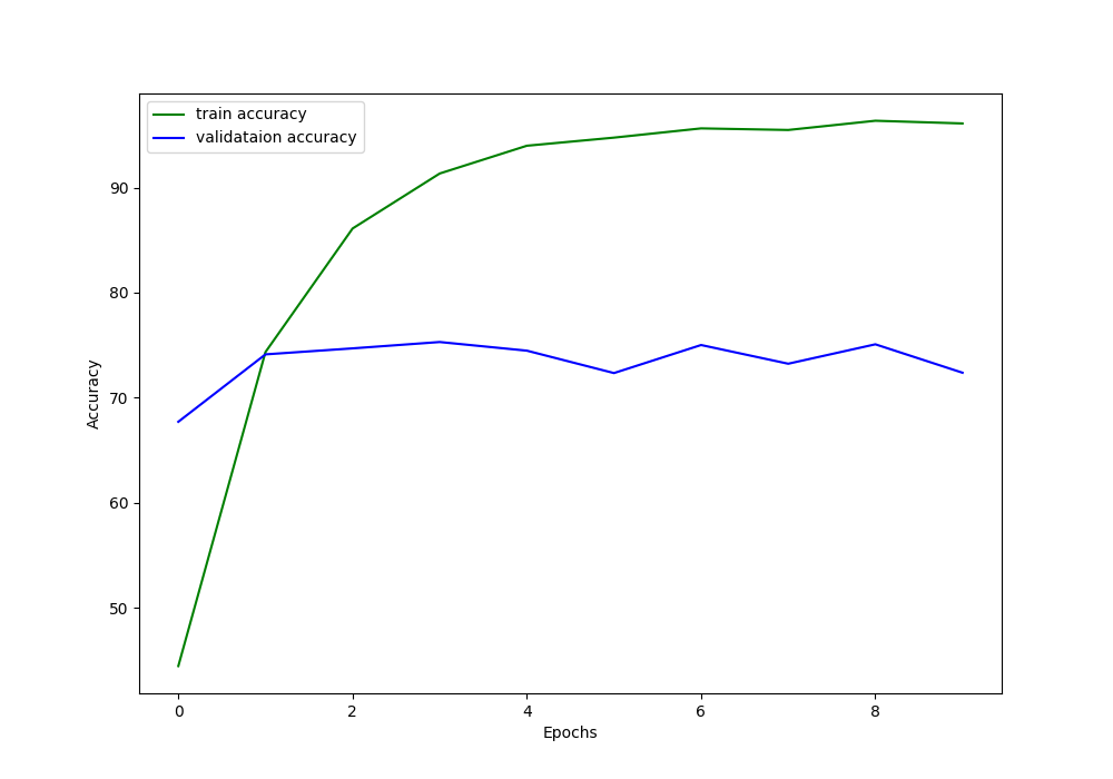
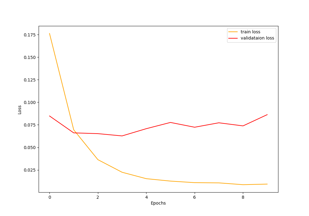
For both, the accuracy and the loss values, overfitting occurs very early. The neural network model starts to overfit just after 3 epochs. Most probably, it is the result of a lack of regularization while training.

Perhaps, employing image augmentation techniques and fine-tuning the head of the model in a better way will prevent overfitting.

I am making a Colab notebook containing the code public here. You can experiment with the code and share the results in the comment section.

Summary and Conclusion

In this article, you learned how an imbalanced image dataset can affect the accuracy of neural network models. The classes with more images get recognized almost correctly. But the classes with fewer images make the accuracy of the neural network model to drop drastically. Regularization techniques like image augmentation might help in such situations. You can share your thoughts in the comment section and I will do my best to address them.

You can contact me using the Contact section. You can also find me on LinkedIn, and Twitter.