Getting 95% Accuracy on the Caltech101 Dataset using Deep Learning

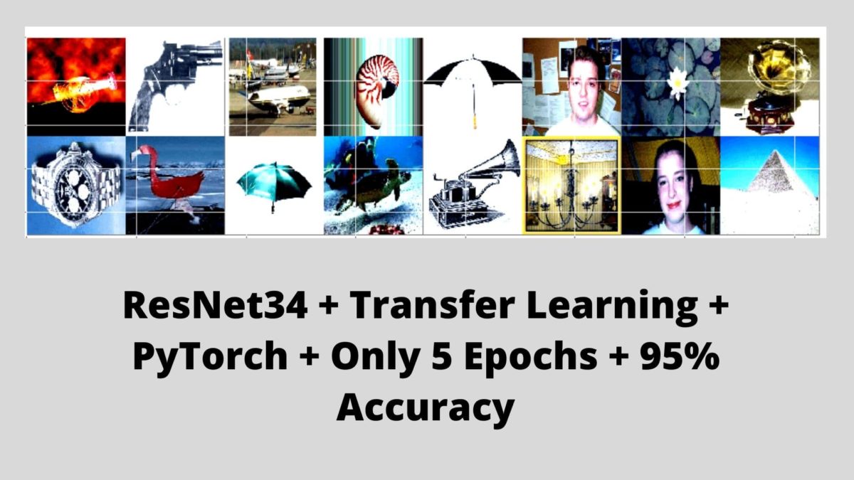
In this article, we will train a ResNet34 deep neural network on the Caltech101 dataset using transfer learning and try to achieve more than 95% test accuracy. The main question is why the Caltech101 dataset for this deep learning tutorial?

In deep learning and training deep neural networks having an imbalanced dataset is a very major problem. And more so, if the dataset is a computer vision dataset. The Caltech101 computer vision dataset is one such imbalanced dataset. And we will try to achieve more than 95% validation and test accuracy using deep learning and neural networks.

What Will We Cover in This Article?

• Knowing about the Caltech101 dataset.
• Our approach to training the deep neural network in this article.
  • The neural network model.
  • Tools and libraries.
  • Directory structure.
• Getting into the code.

The Caltech101 Dataset

As we need to use the Caltech101 dataset in this tutorial, therefore, we first need to download the data.

You can download the Caltech101 dataset from here.

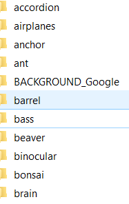
After you download the dataset, then you need to extract it. All the images will be inside subdirectories inside the 101_ObjectCategories folder. The subdirectories names will be the labels in this case. There are actually 102 such subdirectories. One of them is the BACKGROUND_Google subdirectory which we can ignore. We will handle that during the coding, and then we will have 101 labels.

The Image Distribution in the Caltech101 Dataset

If we ignore the BACKGROUND_Google label and its images, then we have 8677 images in total. Now, if you have been doing deep learning for a while, then you will know that these are not enough images to get very high accuracy. Still, we will try our best.

Apart, from the less number of images, another problem is the distribution of the images, per class. According to the official website, there are about 40 to 800 images per category. And most of the categories have around 50 images in the dataset.

Such varying images per category can be a real problem when trying to achieve high accuracy in deep neural network training.

To get a better idea about the distribution of the images in each category, the following image might be useful.

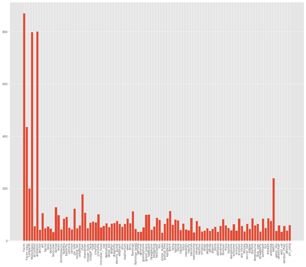
We can clearly see that Faces category has the highest number of images, around 900. And the lowest number of images may be as low as 40. Such an imbalanced dataset is one of the major reasons for the bad performance of deep neural networks.

Approach for Training Our Deep Neural Network

In this section, we will discuss the various aspects of training our deep learning neural network.

The Neural Network Model

We will use ResNet34 for training on the Caltech101 dataset. And we will not be designing the architecture from scratch. In fact, we will be using a pre-trained ResNet34 model with ImageNet weights. So, we will use transfer learning which we know is a really powerful method to gain high-performance improvements in deep learning.

For the hidden layer weights, we will not update them. But we will fine-tune the head of the ResNet34 neural network model to support our use case. While fine-tuning, we will also add a Dropout layer.

Later in the article, we will discuss how this extra dropout layer helps in training and achieving better results.

Getting High Accuracy with the Imbalanced Dataset

We already know that the image distribution per category is imbalanced in our dataset. Traditional approaches in deep learning and more so, in training neural networks use a few of the following approaches to solve the issue:

• Getting more data:
  • This is one of the classic approaches to dealing with an imbalanced image or computer vision datasets. In this approach, we need to collect more data per category which has less number of images. This method works really well as the dataset size can increase substantially. And we know that, when a neural network trains on a larger dataset, then its performance can increase substantially.
• Using Data Augmentation:
  • It is not always possible to get more data. The dataset may be very different from other datasets, or it may be a very new dataset on which many experiments have not been done. In such cases, data augmentation works very well. Data augmentation makes the neural network to see different types of images by changing the images randomly. The changes can be in size, cropping, rotation, color, sharpness, and many more. If you want to learn more practical aspects of image augmentation, then you can visit these articles:
    • Image Augmentation using PyTorch and Albumentations.
    • Adding Noise to Image Data for Deep Learning Data Augmentation.
    • How Useful is Image Augmentation in Deep Learning?.
    • Image Augmentation with Keras for Better Deep Learning.

But we will neither be adding more images to the dataset, nor use data augmentation. In fact, we will only rely upon transfer learning and fine-tuning of the neural network model to achieve higher accuracy.

Above that, we will train the neural network just for 5 epochs to get 95% test accuracy.

Tools and Libraries

We will use the PyTorch deep learning library in this tutorial. Along with that, for the pre-trained ResNet34 neural network model, we will use this great collection of PyTorch pre-trained models. So, you need to install PyTorch and the pre-trained models module for moving further. We will also use the imutils package that will make the extraction of labels from the path names much easier.

• Install PyTorch.
• Install pretraindemodels.
  • pip install pretrainedmodels
• Install imutils
  • pip install imutils

Other packages that we will use are very generic ones that you most probably have. If not, then please do install along the way.

The Directory Structure for This Tutorial

We will use a very simple, yet efficient directory structure to store and save everything.

├───input
│   ├───101_ObjectCategories
│   │   ├───accordion
│   │   ├───airplanes
│   │   ├───anchor
│   │   ├───ant
│   │   ├───BACKGROUND_Google
│   │   ├───barrel
│   │   ├───bass
│   │   ├───beaver
│   │   ├───binocular
│   │   ├───bonsai
│   │   ├───brain
│   │   ├───brontosaurus
...
├───outputs
│   ├───models
│   └───plots
└───src
    └───train.py

• input will contain the 101_ObjectCategories folder which in turn will contain the subdirectories with the images.
• src will contain our train.py file.
• outputs has two directories inside it. models will save the final PyTorch trained model and plots will have the loss and accuracy plots.

Now, let’s start coding our way through this tutorial.

Achieving 95% Accuracy on Caltech101 Dataset using ResNet34 Transfer Learning

From here on, we will write the code that will go into the train.py file inside src.

If you want to directly get into the code, then you can find the colab notebook here.

Importing Modules and Setting the Seed

In this section, we will import all the modules that we need for the tutorial. We will also set the seed for the train.py file. Seeding will help us to reproduce results whenever we want to run this file multiple times.

The following code snippet imports all the needed modules and also sets the seed.

# imports
import matplotlib.pyplot as plt
import matplotlib
import joblib
import cv2
import os
import torch 
import numpy as np
import torch.nn as nn
import torch.nn.functional as F
import torch.optim as optim
import time
import random
import pretrainedmodels

from imutils import paths
from sklearn.preprocessing import LabelBinarizer
from sklearn.model_selection import train_test_split
from torchvision.transforms import transforms
from torch.utils.data import DataLoader, Dataset
from tqdm import tqdm

matplotlib.style.use('ggplot')

'''SEED Everything'''
def seed_everything(SEED=42):
    random.seed(SEED)
    np.random.seed(SEED)
    torch.manual_seed(SEED)
    torch.cuda.manual_seed(SEED)
    torch.cuda.manual_seed_all(SEED)
    torch.backends.cudnn.benchmark = True # keep True if all the input have same size.
SEED=42
seed_everything(SEED=SEED)
'''SEED Everything'''

Going over some of the important imports in the above code block.

• torch.nn will help us access the neural network layers in the PyTorch library.
• torch.optim to access all the optimizer functions in PyTorch.
• pretrainedmodels to access all the pre-trained models like ResNet34 and many more. We installed this library in one of the previous sections.
• Using torchvision.transforms we can apply transforms to our image like normalization and resizing.
• DataLoader and Dataset from the torchvision.transforms will help us to create our own custom image dataset module and iterable data loaders.
• cv2 to read images in the dataset.

Then starting from lines 25 to 35 we apply different seeds for the reproducibility of the results. One of the important ones among these is the torch.backends.cudnn.benchmark. Keeping this True can help us achieve better results. But there is a catch to using this. You should keep this True only if all the input images are of the same size. Else you should keep this False. In the dataset, the image sizes vary. But we will be resizing all the images to 224×224. So, we can keep this True.

Defining the Computation Device, Epochs, and Batch Size

Using a GPU for deep learning can make the neural network training much faster rather than when using CPU. But manually choosing the computation device while writing code is not a very good idea. A simple for loop can automate this.

if torch.cuda.is_available():
    device = 'cuda'
else:
    device = 'cpu'

epochs = 5
BATCH_SIZE = 16

We will be training our model for 5 epochs only, and we are using a batch size of 16. You can use a higher batch size depending upon the amount of GPU memory at your disposal.

Preparing the Labels and Images

The images are inside subdirectories and the names of the subdirectories imply the category the images belong to.

Here, we will prepare the read the images from the folders and create our labels as well.

image_paths = list(paths.list_images('../input/101_ObjectCategories'))

data = []
labels = []
for image_path in image_paths:
    label = image_path.split(os.path.sep)[-2]
    if label == 'BACKGROUND_Google':
        continue

    image = cv2.imread(image_path)
    image = cv2.cvtColor(image, cv2.COLOR_BGR2RGB)

    data.append(image)
    labels.append(label)

data = np.array(data)
labels = np.array(labels)

• image_paths is a list that contains the path to all the images in our dataset (line 1). We will use this list to extract the labels.
• Starting from line 5, we iterate through all the paths in image_paths. Line 6 extracts the directory name of the image which will act as the label for that image. Note that we are ignoring the BACKGROUND_Google images.
• Line 10 reads the image from the path and line 11 converts it to RGB format from the default BGR format of OpenCV.
• Then lines 13 and 14 append each image in the data and labels list respectively.
• Finally, at lines 16 and 17, we convert the data and labels into NumPy arrays.

Next, we will one-hot encode the labels to NumPy array.

# one hot encode
lb = LabelBinarizer()
labels = lb.fit_transform(labels)
print(f"Total number of classes: {len(lb.classes_)}")

We are using LabelBinarizer() from sklearn.preprocessing to one-hot encode the labels.

Define the Image Transforms

In this section, we will define the image transforms that we apply to all the images.

# define transforms
train_transform = transforms.Compose(
    [transforms.ToPILImage(),
	 transforms.Resize((224, 224)),
     transforms.ToTensor(),
     transforms.Normalize(mean=[0.485, 0.456, 0.406],
                          std=[0.229, 0.224, 0.225])])
val_transform = transforms.Compose(
    [transforms.ToPILImage(),
	 transforms.Resize((224, 224)),
     transforms.ToTensor(),
     transforms.Normalize(mean=[0.485, 0.456, 0.406],
                          std=[0.229, 0.224, 0.225])])

In the above code block, we define two transforms. One is train_transform and the other one is val_transform. We will apply the train_transform to our training dataset and val_transform to the validation and test dataset. We are resizing the images to 224×224 pixels, converting them to tensors, and applying normalization as per the pre-trained ImageNet weights.

You can see that both of the transforms are similar. Then why define them separately? This is for those cases when we want to apply some image augmentation to the training set but not to the validation and test set. It is common practice in deep learning and computer vision experiments to apply image augmentations to the training set only. For those situations, if you want to change the train_transform, then you need not touch the val_transform. This will enable us to carry out deep learning experiments very smoothly.

Divide Data into Train, Validation, and Test Set

We will divide our entire dataset into a training set, a validation set, and test data. The distribution is as such: 60% data for training, 20% data for validating, and 20% data for testing.

# divide the data into train, validation, and test set
(X, x_val , Y, y_val) = train_test_split(data, labels, 
                                                    test_size=0.2,  
                                                    stratify=labels,
                                                    random_state=42)

(x_train, x_test, y_train, y_test) = train_test_split(X, Y, 
                                                    test_size=0.25, 
                                                    random_state=42)

print(f"x_train examples: {x_train.shape}\nx_test examples: {x_test.shape}\nx_val examples: {x_val.shape}")

Starting from line 2, first, we reserve 20% of the data for validation. x_val and y_val store the image pixel values, and the corresponding labels respectively.

Then, from line 7, we divide the rest of the data into a training set and test set. Specifically, the number of instance distribution is as the following:

x_train examples: (5205,)
x_test examples: (1736,)
x_val examples: (1736,)

Creating Custom Dataset and Data Loaders

Using the PyTorch Dataset module, we will create our custom dataset module.

We will also create the iterable data loaders in this section.

The following is the custom dataset module.

# custom dataset
class ImageDataset(Dataset):
    def __init__(self, images, labels=None, transforms=None):
        self.X = images
        self.y = labels
        self.transforms = transforms
         
    def __len__(self):
        return (len(self.X))
    
    def __getitem__(self, i):
        data = self.X[i][:]
        
        if self.transforms:
            data = self.transforms(data)
            
        if self.y is not None:
            return (data, self.y[i])
        else:
            return data
        
train_data = ImageDataset(x_train, y_train, train_transform)
val_data = ImageDataset(x_val, y_val, val_transform)
test_data = ImageDataset(x_test, y_test, val_transform)

• In __init__() (line 2), we are initializing the images, labels, and transforms.
• In __getitem__() (line 11), we are returning each image after applying the transforms to it. If the image data has a corresponding label associated with it, then we are returning the label as well. In our case, each of the images has a label.

The next code block defines the data loaders, namely, trainloader, valloader, and testloader.

# dataloaders
trainloader = DataLoader(train_data, batch_size=BATCH_SIZE, shuffle=True)
valloader = DataLoader(val_data, batch_size=BATCH_SIZE, shuffle=True)
testloader = DataLoader(test_data, batch_size=BATCH_SIZE, shuffle=False)

The batch size is 16, as defined previously. We are shuffling the trainloader, and valloader, but not the testloader.

The Neural Network Model

We will use the ResNet34 model from the pretrained models GitHub repository. This repository contains many state-of-the-art convolutional neural network models that we can use very easily.

We will use the ImageNet weights for our ResNet34 model. Also, we will fine-tune the head of the network with an additional dropout layer. Let’s define the ResNet34() module.

# the resnet34 model
class ResNet34(nn.Module):
    def __init__(self, pretrained):
        super(ResNet34, self).__init__()
        if pretrained is True:
            self.model = pretrainedmodels.__dict__['resnet34'](pretrained='imagenet')
        else:
            self.model = pretrainedmodels.__dict__['resnet34'](pretrained=None)
        
        # change the classification layer
        self.l0 = nn.Linear(512, len(lb.classes_))
        self.dropout = nn.Dropout2d(0.4)

    def forward(self, x):
        # get the batch size only, ignore (c, h, w)
        batch, _, _, _ = x.shape
        x = self.model.features(x)
        x = F.adaptive_avg_pool2d(x, 1).reshape(batch, -1)
        x = self.dropout(x)
        l0 = self.l0(x)
        return l0

model = ResNet34(pretrained=True).to(device)

• First, we initialize the ResNet34 model with ImageNet weights (from line 2).
• Then line 11 initializes self.l0 to change the classification layer. The out_features should match the total number of classes. We can access the total number of classes by using len(lb.classes_). We also initialize a Dropout2d() with 0.4 probability.
• The forward() function from line 14 fine-tunes the head of the model. Line 19 applies the dropout just before the fully connected classification layer.

At line 23 we initialize our model and load it onto the computation device.

The next block of code defines the optimizer and the and loss function for our neural network model. We are using the Adam optimizer with a learning rate of 0.0001. And the loss function is cross-entropy loss.

# optimizer
optimizer = optim.Adam(model.parameters(), lr=1e-4)
# loss function
criterion = nn.CrossEntropyLoss()

The Training, Validation, and Test Functions

We will define our three functions for training, validation, and testing here.

The Training Function

Let’s start with the training function.

# training function
def fit(model, dataloader):
    print('Training')
    model.train()
    running_loss = 0.0
    running_correct = 0
    for i, data in tqdm(enumerate(dataloader), total=int(len(train_data)/dataloader.batch_size)):
        data, target = data[0].to(device), data[1].to(device)
        optimizer.zero_grad()
        outputs = model(data)
        loss = criterion(outputs, torch.max(target, 1)[1])
        running_loss += loss.item()
        _, preds = torch.max(outputs.data, 1)
        running_correct += (preds == torch.max(target, 1)[1]).sum().item()
        loss.backward()
        optimizer.step()
        
    loss = running_loss/len(dataloader.dataset)
    accuracy = 100. * running_correct/len(dataloader.dataset)
    
    print(f"Train Loss: {loss:.4f}, Train Acc: {accuracy:.2f}")
    
    return loss, accuracy

• The fit() function takes two input parameters, model and the dataloader. Inside the fit(), we are defining running_loss and running_correct to keep track of batch-wise loss and accuracy.
• For each batch (starting from line 7), we are setting the gradients to zero at line 9 and then getting the outputs.
• After calculating the loss and running_loss, we are getting the predictions at line 13. Then we calculate the running_correct.
• At lines 15 and 16, we backpropagate the gradients and update the gradient parameters.
• After each epoch, we calculate the loss and accuracy and print them as well. And we are returning the loss and accuracy for each epoch as well.

The Validation Function

The validation function is going to be very similar to the training function, except for a few changes.

#validation function
def validate(model, dataloader):
    print('Validating')
    model.eval()
    running_loss = 0.0
    running_correct = 0
    with torch.no_grad():
        for i, data in tqdm(enumerate(dataloader), total=int(len(val_data)/dataloader.batch_size)):
            data, target = data[0].to(device), data[1].to(device)
            outputs = model(data)
            loss = criterion(outputs, torch.max(target, 1)[1])
            
            running_loss += loss.item()
            _, preds = torch.max(outputs.data, 1)
            running_correct += (preds == torch.max(target, 1)[1]).sum().item()
        
        loss = running_loss/len(dataloader.dataset)
        accuracy = 100. * running_correct/len(dataloader.dataset)
        print(f'Val Loss: {loss:.4f}, Val Acc: {accuracy:.2f}')
        
        return loss, accuracy

• Notice that we are setting model.eval() for validation first.
• Moreover, everything is taking place inside the with torch.no_grad() block. This is important so that the gradients do not get calculated as we do not them during validation.
• Also, we are not zeroing, or backpropagating, or updating any gradients.

The Test Function

The test function is a very simple one.

def test(model, dataloader):
    correct = 0
    total = 0
    with torch.no_grad():
        for data in testloader:
            inputs, target = data[0].to(device), data[1].to(device)
            outputs = model(inputs)
            _, predicted = torch.max(outputs.data, 1)
            total += target.size(0)
            correct += (predicted == torch.max(target, 1)[1]).sum().item()

    return correct, total

• In the test() function, we are calculating the total number of inputs, and the total number of images that our model predicts correctly. We return those finally at line 12.

Training Our Neural Network Model

For training the neural network model, we will call the fit() and validate() functions for 5 epochs. A simple for loop will work nicely here.

We will save the epoch-wise losses in train_loss and val_loss, and the accuracies in train_accuracy and val_accuracy. These four will be lists.

train_loss , train_accuracy = [], []
val_loss , val_accuracy = [], []
print(f"Training on {len(train_data)} examples, validating on {len(val_data)} examples...")
start = time.time()
for epoch in range(epochs):
    print(f"Epoch {epoch+1} of {epochs}")
    train_epoch_loss, train_epoch_accuracy = fit(model, trainloader)
    val_epoch_loss, val_epoch_accuracy = validate(model, valloader)
    train_loss.append(train_epoch_loss)
    train_accuracy.append(train_epoch_accuracy)
    val_loss.append(val_epoch_loss)
    val_accuracy.append(val_epoch_accuracy)
end = time.time()
print((end-start)/60, 'minutes')

torch.save(model.state_dict(), f"../outputs/models/resnet34_epochs{epochs}.pth")

# accuracy plots
plt.figure(figsize=(10, 7))
plt.plot(train_accuracy, color='green', label='train accuracy')
plt.plot(val_accuracy, color='blue', label='validataion accuracy')
plt.xlabel('Epochs')
plt.ylabel('Accuracy')
plt.legend()
plt.savefig('../outputs/plots/accuracy.png')

# loss plots
plt.figure(figsize=(10, 7))
plt.plot(train_loss, color='orange', label='train loss')
plt.plot(val_loss, color='red', label='validataion loss')
plt.xlabel('Epochs')
plt.ylabel('Loss')
plt.legend()
plt.savefig('../outputs/plots/loss.png')

• We are also tracking the time it takes to train the whole neural network for 5 epochs (starting at line 4 and ending at line 13). If you have a GPU, then the training will finish very fast.
• After each epoch, we are appending the losses and accuracies to the respective loss and accuracy lists.
• Line 16 saves the model as a .pth file. You can load this model and use it in the future whenever you want.
• The rest of the code is for saving the loss and accuracy plots. We are saving those plots in outputs/plots. We will analyze the plot results shortly.

It is also a good idea to save the accuracy and loss lists as pickled files. We do not want to lose our results once we finish running/training our model. Saving them as .pkl files will help us load them whenever we want them and use them as simple lists again.

# save the accuracy and loss lists as pickled files
print('Pickling accuracy and loss lists...')
joblib.dump(train_accuracy, '../outputs/models/train_accuracy.pkl')
joblib.dump(train_loss, '../outputs/models/train_loss.pkl')
joblib.dump(val_accuracy, '../outputs/models/val_accuracy.pkl')
joblib.dump(val_loss, '../outputs/models/val_loss.pkl')

For example, the following code will load the train_accuacy again as a list.

train_acc = joblib.load('../outputs/models/train_accuracy.pkl')

Testing Our Neural Network Model

Now is the time to test our deep neural network model. We just need to call the test() function while passing the model and testloader as arguments.

correct, total = test(model, testloader)
print('Accuracy of the network on test images: %0.3f %%' % (100 * correct / total))
print('train.py finished running')

Finally, we print the accuracy on the test set.

Let’s run the train.py file and see the results that we get.

Running the train.py File

From inside the src/ folder, type the following command in your terminal.

python train.py

The following is a short snippet of the whole output.

Total number of classes: 101
x_train examples: (5205,)
x_test examples: (1736,)
x_val examples: (1736,)
Training on 5205 examples, validating on 1736 examples...
Epoch 1 of 5
Training
326it [00:53,  6.05it/s]
Train Loss: 0.1033, Train Acc: 67.49
Validating
109it [00:08, 13.03it/s]
Val Loss: 0.0237, Val Acc: 91.65
...
Epoch 5 of 5
Training
326it [00:54,  5.96it/s]
Train Loss: 0.0035, Train Acc: 99.21
Validating
109it [00:08, 12.73it/s]
Val Loss: 0.0130, Val Acc: 94.35
5.1683531403541565 minutes
Pickling accuracy and loss lists...
Accuracy of the network on test images: 95.104 %
train.py finished running

As you can see, the neural network model is getting 95.1% accuracy on the test set. The results may vary anything between 95% and 96% on different runs. But on average, the neural network will be 95% accurate.

One of the main reasons for the high accuracy in a very small number of training epochs is the additional dropout layer. You will observe that removing the dropout layer before the fully connected layer will give you worse results.

Analyzing the Plots and Results

Let’s take look at the accuracy plot first.

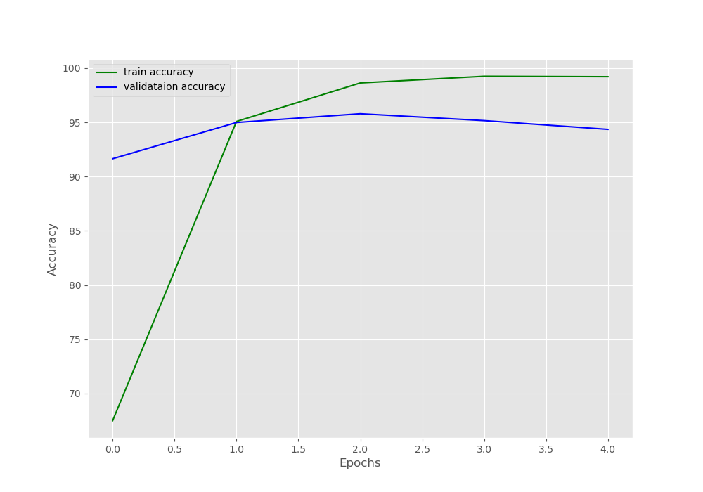
We can see that the model starts to overfit after two epochs. Training any longer will lead to a serious drop in the validation accuracy.

Now, let’s take a look at the loss plot.

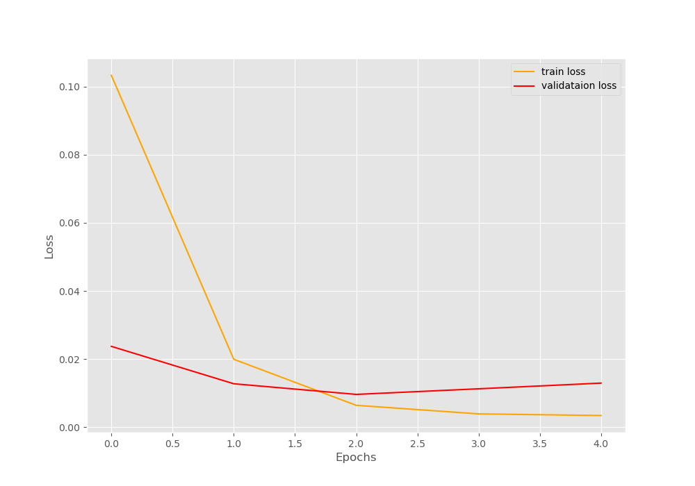
The loss values also have a similar story. The neural network model starts to show an increase in loss values after 2 epochs. A classic indication of the neural network overfitting.

How to Overcome Overfitting When Training Deep Neural Network Model?

As we saw above, our neural network model gives very high accuracy in just 5 epochs but starts to overfit as well.

The main reason behind it is the small number of images that we have in the dataset. The Caltech101 dataset has only around 8700 images. The neural network model is ResNet34 which a very large and powerful model.

Now, using a smaller network like ResNet18 may give us a more robust model after training. But what if we want to have a robust model using ResNet34 only?

The best way to reduce overfitting, and train a more robust deep neural network model is to use image augmentation. Image augmentation can include flipping, rotating, cropping, changing the color palette and many more operations.

Augmenting the images will make the neural network model see different types of images. This adds a regularizing effect as well which prevents overfitting and makes the network robust to augmented images during test time as well.

But when using image augmentation, then you will need to train the neural network for longer to achieve higher accuracy. Be sure to post your findings in the comment section if you try out image augmentation.

you can find the colab notebook here. You can also try out image augmentation directly in the notebook.

Summary and Conclusion

In this article, you learned how to train a ResNet34 neural network model on the Caltech101 dataset. You learned how to fine-tune the head of a model to gain high accuracy in just a few epochs. Overfitting was a major problem in this case. Leave your thoughts in the comment section and I will try my best to address them.

You can contact me using the Contact section. You can also find me on LinkedIn, and Twitter.