How Useful is Image Augmentation in Deep Learning?

In this article, we will take a look at how we can use image augmentation in deep learning.

Data augmentation is a very useful technique when dealing with image data. Image augmentation is most helpful when the dataset is small. We can also benefit from image augmentation when we are not able to find any more images for training a neural network model.

But actually how useful are image augmentation techniques? Do they really benefit while training a neural network model on a dataset? We will try to find the answer to these questions in this article.

You can read this article to know the various types of image augmentation techniques.

So, in this article, we will take a look at the usefulness of image augmentation in deep learning when building an image classifier.

The Dataset

For this article, we will be using the CIFAR10 dataset. We will need to compare our models with and without augmentation. For that CIFAR10 will provide us a good amount of complexity.

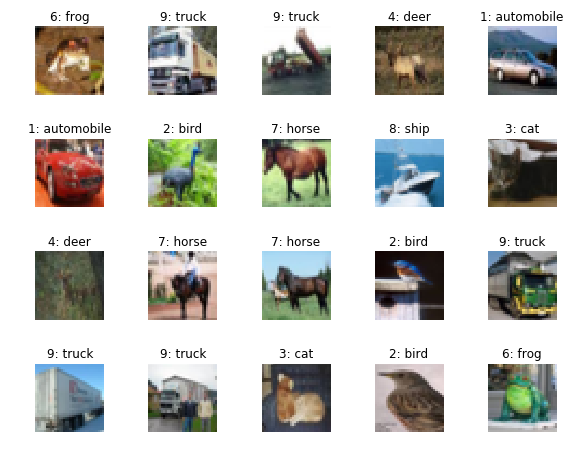
The CIFAR10 dataset contains 60000 labeled images distributed among 10 classes. So, there are 6000 images belonging to each class. The following are the label classes in the dataset:
airplane
automobile 
bird 
cat 
deer 
dog 
frog 
horse 
ship 
truck

We will use the Keras module from TensorFlow, that is the tf.keras module.

Why CIFAR10?

Many of you may be thinking about why I have chosen the CIFAR10 dataset for this article. There are many other simpler datasets like the digit MNIST or the Fashion MNIST.

It is true that we will be able to produce the results faster with those datasets. But we will not able to apply some augmentation techniques like flipping and rotating properly to the digit MNIST. That’s because flipping or rotating the numbers may result in some orientation problems while classifying. This is mainly true for digits like 6 and 9.

CIFAR10 dataset contains real-life images as you have seen above.It will allow us to apply enough data augmentation techniques without thinking much about rotation or orientation problems. That’s why I thought that CIFAR10 will be most appropriate for this article.

If you have any other ideas or think differently, let me know in the comment section. I will be happy to get new ideas. I will be happy to consider and address them.

Let’s get started.

Necessary Imports and Data Preparation

First, let’s import all the necessary packages and modules that we will need along the way.

import numpy as np
import tensorflow as tf
import seaborn as sns
import matplotlib.pyplot as plt

from tensorflow import keras

Before downloading the dataset, let’s define the constants for batch size and the number of epochs.

BATCH_SIZE = 32
N_EPOCHS = 100

We will train our neural network model for 100 epochs.

We can download the CIFAR10 dataset directly from keras.datasets module.

(x_train, y_train), (x_test, y_test) = keras.datasets.cifar10.load_data()

print('x_train shape:', x_train.shape)
print(x_train.shape[0], 'samples for training')
print(x_test.shape[0], 'samples for testing')

x_train shape: (50000, 32, 32, 3)
50000 samples for training
10000 samples for testing

In the dataset, we have 60000 images in total. From those 60000, 50000 images are for training and 10000 are for testing purposes.

Now, let’s normalize our image NumPy arrays for both training and testing sets. Along with that, we will also convert the labels into binary class matrices using keras.utils.to_categorical.

x_train = x_train.astype('float32') / 255
x_test = x_test.astype('float32') / 255

# class vectors to binary class matrices
y_train = keras.utils.to_categorical(y_train, num_classes=10)
y_test = keras.utils.to_categorical(y_test, num_classes=10)

Building the Model

Next, we will stack up the layers of our neural network model. For that, we will define a function, build_model. Defining a function will help us to build our model easily.

We will need to build two models. One we will train without any image augmentation and one with image augmentation.

def build_model():
    model = keras.models.Sequential()
    model.add(keras.layers.Conv2D(32, (3, 3), padding='same',
                 input_shape=(32, 32, 3)))
    model.add(keras.layers.Activation('relu'))
    model.add(keras.layers.BatchNormalization())
    model.add(keras.layers.Conv2D(32, (3, 3), padding='same'))
    model.add(keras.layers.Activation('relu'))
    model.add(keras.layers.BatchNormalization())
    model.add(keras.layers.MaxPooling2D(pool_size=(2, 2)))
    model.add(keras.layers.Dropout(0.25))

    model.add(keras.layers.Conv2D(64, (3, 3), padding='same'))
    model.add(keras.layers.Activation('relu'))
    model.add(keras.layers.BatchNormalization())
    model.add(keras.layers.Conv2D(64, (3, 3), padding='same'))
    model.add(keras.layers.Activation('relu'))
    model.add(keras.layers.BatchNormalization())
    model.add(keras.layers.MaxPooling2D(pool_size=(2, 2)))
    model.add(keras.layers.Dropout(0.25))

    model.add(keras.layers.Conv2D(128, (3, 3), padding='same'))
    model.add(keras.layers.Activation('relu'))
    model.add(keras.layers.BatchNormalization())
    model.add(keras.layers.Conv2D(128, (3, 3), padding='same'))
    model.add(keras.layers.Activation('relu'))
    model.add(keras.layers.BatchNormalization())
    model.add(keras.layers.MaxPooling2D(pool_size=(2, 2)))
    model.add(keras.layers.Dropout(0.4))

    model.add(keras.layers.Flatten())
    model.add(keras.layers.Dense(10))
    model.add(keras.layers.Activation('softmax'))

    # initiate RMSprop optimizer
    opt = keras.optimizers.RMSprop(lr=0.001, decay=1e-6)

    # compile the model
    model.compile(loss='categorical_crossentropy',
                optimizer=opt,
                metrics=['accuracy'])
    
    return model

To build our neural network model, we just need to call the build_model() function.

To build our model we have stacked up Conv2D layers with 32, 64 and 128 output dimensionality respectively. All the convolutional Conv2D layers are followed by Activation('relu') layers.

The MaxPooling2D have a pool size of (2, 2). All the Dropout layers have a dropout rate of 0.25 except for the last one, where it is 0.4.

Finally, we use Flatten() and Dense() layers with 10 output dimensionality. For compiling we have used RMSprop() optimizer.

Let’s move on to train our network without any augmentation.

Training Without Image Augmentation

First, we need to build our model.

model_1 = build_model()
print(model_1.summary())

_________________________________________________________________
Layer (type)                 Output Shape              Param #   
=================================================================
conv2d (Conv2D)              (None, 32, 32, 32)        896       
_________________________________________________________________
activation (Activation)      (None, 32, 32, 32)        0         
_________________________________________________________________
batch_normalization (BatchNo (None, 32, 32, 32)        128       
_________________________________________________________________
conv2d_1 (Conv2D)            (None, 32, 32, 32)        9248      
_________________________________________________________________
activation_1 (Activation)    (None, 32, 32, 32)        0         
_________________________________________________________________
batch_normalization_1 (Batch (None, 32, 32, 32)        128       
_________________________________________________________________
max_pooling2d (MaxPooling2D) (None, 16, 16, 32)        0         
_________________________________________________________________
dropout (Dropout)            (None, 16, 16, 32)        0         
_________________________________________________________________
conv2d_2 (Conv2D)            (None, 16, 16, 64)        18496     
_________________________________________________________________
activation_2 (Activation)    (None, 16, 16, 64)        0         
_________________________________________________________________
batch_normalization_2 (Batch (None, 16, 16, 64)        256       
_________________________________________________________________
conv2d_3 (Conv2D)            (None, 16, 16, 64)        36928     
_________________________________________________________________
activation_3 (Activation)    (None, 16, 16, 64)        0         
_________________________________________________________________
batch_normalization_3 (Batch (None, 16, 16, 64)        256       
_________________________________________________________________
max_pooling2d_1 (MaxPooling2 (None, 8, 8, 64)          0         
_________________________________________________________________
dropout_1 (Dropout)          (None, 8, 8, 64)          0         
_________________________________________________________________
conv2d_4 (Conv2D)            (None, 8, 8, 128)         73856     
_________________________________________________________________
activation_4 (Activation)    (None, 8, 8, 128)         0         
_________________________________________________________________
batch_normalization_4 (Batch (None, 8, 8, 128)         512       
_________________________________________________________________
conv2d_5 (Conv2D)            (None, 8, 8, 128)         147584    
_________________________________________________________________
activation_5 (Activation)    (None, 8, 8, 128)         0         
_________________________________________________________________
batch_normalization_5 (Batch (None, 8, 8, 128)         512       
_________________________________________________________________
max_pooling2d_2 (MaxPooling2 (None, 4, 4, 128)         0         
_________________________________________________________________
dropout_2 (Dropout)          (None, 4, 4, 128)         0         
_________________________________________________________________
flatten (Flatten)            (None, 2048)              0         
_________________________________________________________________
dense (Dense)                (None, 10)                20490     
_________________________________________________________________
activation_6 (Activation)    (None, 10)                0         
=================================================================
Total params: 309,290
Trainable params: 308,394
Non-trainable params: 896
_________________________________________________________________

Okay, now we are ready to train our neural network. We will train the network for 100 epochs. Remember that we have taken the BATCH_SIZE to be 32. If you somehow run into an OOM (Out of Memory) error, then consider reducing the batch size. It would be better to keep it a power of 2, like 8 or 16.

Also, we consider the whole x_test and y_test as the validation data while training. We want an ample amount of validation data so that our network gets to validate a number of images rather than just a few.

history = model_1.fit(x_train, y_train, 
            validation_data=(x_test, y_test),
            batch_size=BATCH_SIZE,
            epochs=N_EPOCHS)

After the training is complete we can plot the accuracy and loss graphs from the history object. The following code will plot the graphs and save a PNG file of the graph as well.

num_epochs = np.arange(0, N_EPOCHS)
plt.style.use('ggplot')
plt.figure(figsize=(12, 8))
plt.plot(num_epochs, history.history['loss'], label='train_loss', c='red')
plt.plot(num_epochs, history.history['val_loss'], 
    label='val_loss', c='orange')
plt.plot(num_epochs, history.history['acc'], label='train_acc', c='green')
plt.plot(num_epochs, history.history['val_acc'], 
    label='val_acc', c='blue')
plt.title('Training Loss and Accuracy')
plt.xlabel('Epoch')
plt.ylabel('Loss/Accuracy')
plt.legend()
plt.savefig('Images/plot_without_aug.png')

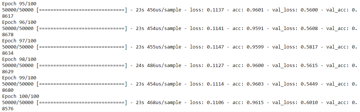
The following image shows the last five epochs of training our neural network.

Let’s take a look at the accuracy and loss plots.

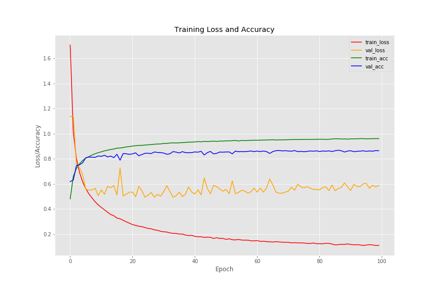
The training accuracy reached almost 96% which is good actually. And the validation accuracy did not rise above 86%.

The story for the loss values is something entirely different. The training loss is around 0.1. It is very clear that we are not getting a smooth decrease in validation loss. We can see a lot of fluctuations. The lowest for the validation loss is between 0.5 and 0.6.

Hopefully, we will do better when using image augmentation while training.

Training with Image Augmentation

In this section, we will build a new model by calling the build_model() function.

We will use image augmentation for the training dataset. But we will not use any augmentation for the test set. When using augmentation for the test set, it also called Test Time Augmentation (TTA) as well. This is mainly done so that the images that the model gets for testing are a bit different as well. But we will skip TTA.

First, let’s define our augmentation arguments for the ImageDataGenerator().

augmentation = keras.preprocessing.image.ImageDataGenerator(rotation_range=15,
	width_shift_range=0.1, height_shift_range=0.1,
	horizontal_flip=True, fill_mode="nearest")

augmentation.fit(x_train)

The following is a brief explanation of the augmentations that we are performing.
rotation_range: this takes an input between 0 and 180 and rotates the image by a certain degree (15 in our case).
width_shift_range and height_shift_range: to shift the images width-wise and height-wise respectively. The input is a floating number between 0.0 and 1.0.
horizontal_flip: this flips the image horizontally. Either True or False.
fill_mode: this specifies how the boundaries of the inputs are filled. By default it is nearest.

Finally, we fit the image data generator on our training data.

If you want to get a full list of tf.keras.preprocessing.image.ImageDataGenerator, then be sure to check out this link.

Now, we are ready to build and train our model. This part is very similar to the one we did without any augmentation. The only real difference is that we will use fit_generator() instead of fit() to train our network.

model_2 = build_model()

history = model_2.fit_generator(augmentation.flow(x_train, y_train,
                                                   batch_size=BATCH_SIZE),
                                                   epochs=N_EPOCHS,
                                                   validation_data=(x_test, y_test))

Observe that we have provided augmentation.flow() method and passed our training data and labels as arguments.

And following the code for accuracy and loss plots.

num_epochs = np.arange(0, N_EPOCHS)
plt.style.use('ggplot')
plt.figure(figsize=(12, 8))
plt.plot(num_epochs, history.history['loss'], label='train_loss', c='red')
plt.plot(num_epochs, history.history['val_loss'], 
    label='val_loss', c='orange')
plt.plot(num_epochs, history.history['acc'], label='train_acc', c='green')
plt.plot(num_epochs, history.history['val_acc'], 
    label='val_acc', c='blue')
plt.title('Training Loss and Accuracy')
plt.xlabel('Epoch')
plt.ylabel('Loss/Accuracy')
plt.legend()
plt.savefig('Images/plot_with_aug.png')

The following image shows the last few epochs of training our neural network model.

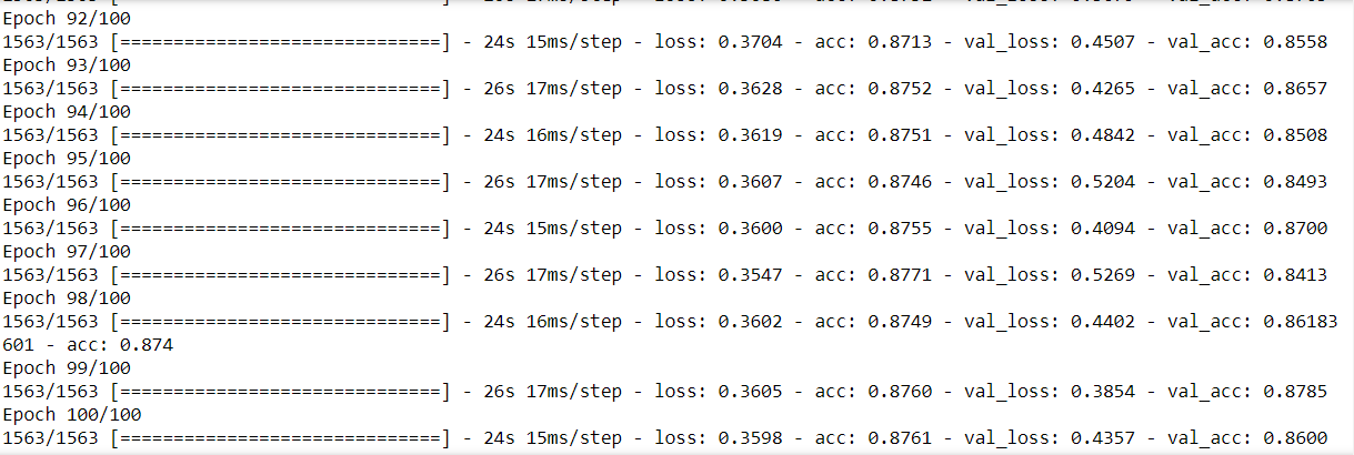
You can see that in the last few epochs we are getting a training accuracy of around 88%. The validation accuracy stays close to 86% mainly but reaches almost 88% in epoch 99. Most probably the network will get even better if trained for more epochs.

Looking at the plots of accuracies and losses.

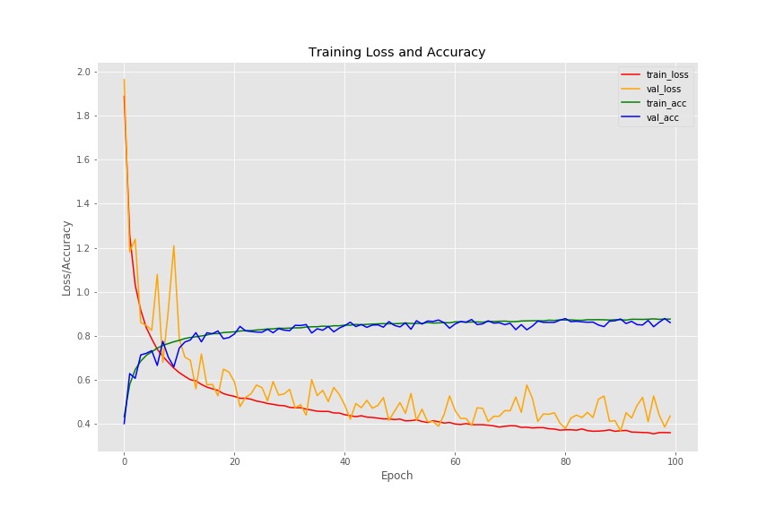
We can see fluctuations in both loss and accuracy lines for validation data. The lowest loss and highest accuracy are matching by the way. In epoch 99 we are getting 0.3854 validation loss and almost 88% validation accuracy. This is a good sign actually. This means that our model made low errors on a few data.

Summary and Conclusion

There are some key takeaways from this article.

First: it is possible to achieve high accuracy without image augmentation as well. But training for longer without augmentation may lead to overfitting.
Second: image augmentation helps to reduce the difference between the training and validation loss and accuracy.
Third: with image augmentation, we can train for more number of epochs without overfitting. Validation accuracy will increase gradually. Also, learning is slower when implementing augmentation. There is obviously a tradeoff between accuracy and training time.

If you found this article useful, then leave your thoughts in the comment section and consider subscribing to the website. Also, you can reach out to me on LinkedIn and Twitter.