Denoising Text Image Documents using Autoencoders

Updated: March 25, 2020.

In this post, we will be denoising text image documents using deep learning autoencoder neural network. And we will not be using MNIST, Fashion MNIST, or the CIFAR10 dataset.

In fact, we will be using one of the past Kaggle competition data for this autoencoder deep learning project. More specifically, we will be using the data from Denoising Dirty Documents competition in this article. This is going to be a lot of fun and you will learn a lot as well.

What Will We Conver in this Article?

• Getting the Data from Kaggle.
  • Downloading and knowing about the data.
• Setting up the project directory.
• Preparing the data:
  • Preparing custom datasets and getting the iterable data loaders.
• Building the autoencoder neural network.
• Training the data.
• Testing the data.

Looks like we have a lot to cover in this article. But still, we will have lots of fun working with this dataset.

So, let’s start.

Getting the Data from Kaggle

I hope that the following steps are very familiar to you. In fact, you may even skip the first step if you already know how to get the data from Kaggle. Still, this part will help any newcomer in this field. So, bear with me if you find the steps redundant.

The first step is to get the data from Kaggle. I hope that you already have a Kaggle account. If not please sign up for a Kaggle account and then we can proceed smoothly.

Ok, after signing up, we can now get the data from Kaggle. To get the data, first, you will accept the competition rules. For that, go over to the competition page and click on the Rules tab. Then simply accept the rules of the competition. You should be seeing the following message.

Next, you can go over to the Data tab and download the dataset. Although, we do not the sampleSubmission.csv file, still you can download it if you intend to submit your results in the future.

Getting to Know the Data

Apart from the sampleSubmission.csv we have three zip files.

• train.zip contains the images that we will train our deep learning autoencoder on. These images contain text to which noise has been added. Our aim is to build an autoencoder neural network that will denoise those images.
• test.zip contains the images that we will use to test our neural network once it has been trained. We will try to get clean images as the output by cleaning the noise from the test images.
• train_cleaned.zip contains the same images as the train images but without the noise. We will use these images as targets to train our network.

So, we will train a supervised autoencoder to be more specific. We will train our autoencoder neural network on the noisy train images. While doing so, we will try to eliminate the noise by posing the clean train image as the targets. After that, when we feed our network with the noisy test images, we should be able to get clean images as output. Just one more thing, we will not be submitting any predictions on to Kaggle. We will just test our network on the noisy test images.

Next, we are all set to set up our project directory.

Setting up the Project Directory

The project directory will consist of three main directories which will, in turn, contain other subdirectories and files. The following is the project directory setup that you probably should carry out before moving further. This will ease out many of our tasks further on.

├───input
│   ├───test
│   ├───train
│   └───train_cleaned
├───models
│   └───Saved_Images
└───src

Breaking down the directory structure:

• input directory contains all the data. This includes train images,test images, and train_cleaned images.
• models will contain any trained model that we will save along with all the output images and visualization.
• src contains all the source code files. You can either use python notebooks (.ipynb) or .py files to write the code. I have tried my best to make the code work in both formats.
• We will be creating the Saved_Images directory in the code only. This is because, we need this the saved images for this project. When using this template, our requirements may change according to projects.

I think we are ready to start the code part of this project.

Denoising Documents using Deep Denoising Autoencoder

Imports and Visualizing the Images

Here, we will import all the Python and PyTorch modules that we will need for this project.

import numpy as np
import pandas as pd
import matplotlib.pyplot as plt
import cv2
import os
import torch
import torchvision
import glob
import torch.nn as nn
import torch.optim as optim
import torch.nn.functional as F

from torchvision.transforms import transforms
from torch.utils.data import Dataset, DataLoader
from torchvision.utils import save_image

Some of the important modules that we have imported are:

• torchvision: helps in carrying out many deep learning related computer vision tasks easily.
• Dataset: the Dataset class will help us create our custom dataset for the images that we have. We will need to override two of its functions, __len__(), and __getitem__().
• DataLoader: this class will help us to create iterable data loaders that we can feed into our autoencoder network for training and testing.

Note: If you have not created any custom dataset using PyTorch before, then you find one of my previous article very useful in this regard. Please take a look at this before moving further. This will help you understand many of the dataset creation concepts much more easily.

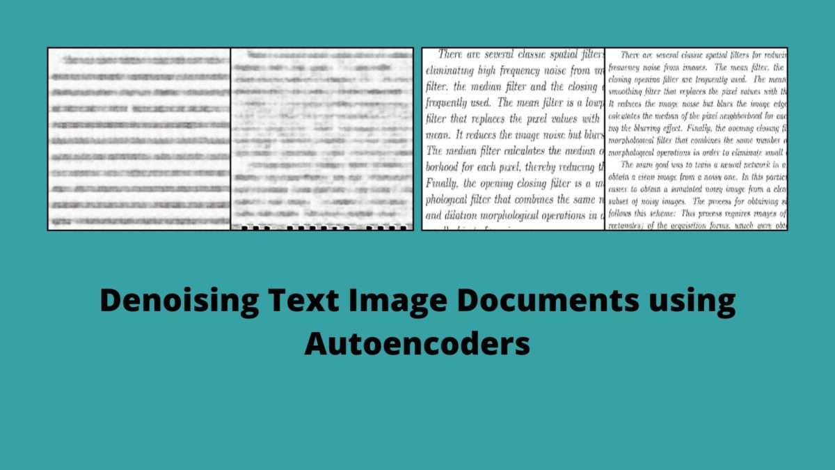
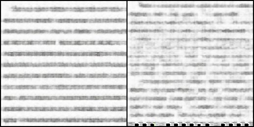
Before moving further into the technical details of the project, let’s take a look at the images that we have. Remember that for training we have both, the noisy images as well the corresponding clean images.

# visualize train images
def show_image(path):
    plt.figure(figsize=(10, 7))
    img = cv2.imread(path)
    print(img.shape)
    plt.imshow(img)
    plt.show()
    
# noisy train image and the corresponding clean train image
show_image('../input/train/2.png')
show_image('../input/train_cleaned/2.png')

The above code will give the following output.

The first image shows the noisy image from the train directory. And the second image shows the corresponding clean image from the train_cleaned directory. You can see that the first image contains a lot of background noise. So, our job will be to train a deep autoencoder neural network to achieve results very similar to the second image.

You can also explore the data more on your own if you want. For now, we will now move on to the preparation of the dataset.

Preparing Custom Dataset and DataLoaders

In this section, we will create a Python class for the custom dataset. This dataset will help us to get the iterable data loaders.

The first step here is to read the data.

TRAIN_IMAGES = glob.glob('../input/train/*.png') 
TRAIN_CLEAN = glob.glob('../input/train_cleaned/*.png')
TEST_IMAGES = glob.glob('../input/test/*.png')

In the above code block, we are using the python glob module to get the .png images from all the thee directories. So, TRAIN_IMAGES, TRAIN_CLEAN, and TEST_IMAGES will contain the names of path from train, train_cleaned, and test directories respectively. They are all lists that just contain the names of the images.

Now, we have to convert those into a more usable format.

Resizing and Saving the Pixel Values

To be able to use the image data properly, we will have to get their pixels values. For that, we will be using the following code.

def get_data(path):
    images = []
    for i, image in enumerate(path):
        image = cv2.imread(image)
        image = cv2.resize(image, (256, 256))
        image = np.reshape(image, image.shape[0]*image.shape[1]*image.shape[2])
        images.append(image)
    return images

x_train = get_data(TRAIN_IMAGES)
y_train = get_data(TRAIN_CLEAN)
x_test = get_data(TEST_IMAGES)

We create a function called get_data() (lines 1 to 8) which takes the path list as the parameter. Starting from line 3 we iterate through the image list. Then from lines 4 – 5 we read the image and resize it to 256×256 pixels. At line 7 we reshape the image and flatten it. This is an important step as it makes the pixel values to be a single row list with all the pixel values. Finally, at line 8 we append the flattened pixels to the images list and return the images. There is also another point to note here. By default, the images have 3 channels, so, we will be writing all the code with respect to that only.

Starting from line 10 till 12 we call the get_data() function three times. Each time we provide a different image list as the argument and save the pixel values in x_train, y_train, and x_test. You can see that we have named the clean images as y_train. This is because we will be using them as the target labels while training.

Printing the length of the three lists we get the following output.

print(len(x_train))
print(len(y_train))
print(len(x_test))

print(x_train[1])

144
144
72

[231 231 231 ... 220 220 220]

So, x_train contains 144 rows, which is equal to the 144 images in the train directory. Now each of those rows contains 256x256x3 = 196608 pixels as the features. Similarly, for the y_train and x_test.

Defining Constants and the Image Transforms

The code in this section will ease out the task of training and testing our model. We will define some constants that we can use easily.

Starting with the constants.

# constants
NUM_EPOCHS = 100
LEARNING_RATE = 1e-3
BATCH_SIZE = 2

We define the number of epochs that we will train the autoencoder neural network for, which is 100. The learning rate is 0.001, and the batch size 2. A batch size of 2 is a safe option here as 256×256 images will take a lot of memory. Along with that when we load the autoencoder network to the GPU as well, that will amount even more. You are free to increase the batch size if you have more GPU memory at your disposal.

The following code defines the image transforms that we will use on the pixel values.

# define transforms
transform = transforms.Compose([
     transforms.ToPILImage(),
     transforms.ToTensor()
])

First, we convert the pixel values into PIL image format on line 3. Then at line 4, we convert the values to tensor. Converting the values to tensors is a very important step in the PyTorch framework. This ensures the correct input format of the data while training and testing.

Writing Custom Dataset Class

In this section, we will write a class ImageData(). This will inherit all the properties of the PyTorch Dataset class. Also, we will be overriding the __len__() and __getitem__() functions as per our requirements.

# prepare the dataset and the dataloader
class ImageData(Dataset):
    def __init__(self, images, labels=None, transforms=None):
        self.X = images
        self.y = labels
        self.transforms = transforms
         
    def __len__(self):
        return (len(self.X))
    
    def __getitem__(self, i):
        data = self.X[i][:]
        data = np.asarray(data).astype(np.uint8).reshape((256, 256, 3))
        
        if self.transforms:
            data = self.transforms(data)
            
        if self.y is not None:
            labels = self.y[i][:]
            labels = np.asarray(labels).astype(np.uint8).reshape((256, 256, 3))
            labels = self.transforms(labels)
            return (data, labels)
        else:
            return data
        
train_data = ImageData(x_train, y_train, transform)
test_data = ImageData(x_test, None, transform)

train_loader = DataLoader(train_data, batch_size=BATCH_SIZE, shuffle=True)
test_loader = DataLoader(test_data, batch_size=BATCH_SIZE, shuffle=True)

When starting the ImageData() class, first we inherit all the properties of the PyTorch Dataset class. The following is the breakdown of the functions inside the ImageData() class:

• __init__(): this is where the execution begins (lines 3 to 6). It takes three input parameters. Out of those, labels and transforms are None by default. This is for those cases where we do not have labels or do not want to apply the transforms to the pixels. Mostly used for preparing the test set. Lines 4, 5, and 6 initialize the images as self.X, labels as self.y, and transforms as self.transforms respectively.
• __len__(): here we just return the length of the dataset. This is equal to the number of samples present in the dataset.
• __getitem__(): in general, this function returns a sample from the dataset when we provide it with an index value. In our case, first, it stores all the data elements in data at line 12. We will have to use a convolutional network that takes 2D input. Therefore, at line 13, we convert the data into a NumPy array and reshape the pixels in each row into 256x256x3. Then at lines 15 and 16, we apply the transforms to the dataset. Now, note that our target labels are also image pixel values. Therefore, starting from line 18 till 21 we apply the same approach to self.y as we have done to data. Finally, we return the data along with the labels at line 22. For the test set, where we do not have any labels, we just return the data at line 24.
• At lines 26 and 27, we create two objects of the ImageData() class. They aretrain_data, and test_data which contains the data as per the execution of the ImageData class.
• Finally, in lines 29 and 30, we create the data loaders of the train_data and test_data. They are train_loader, and test_loader. We use the PyTorch DataLoader module for that. In this case, the batch size is 2 for the data loaders.

Writing Helper Functions

As for the helper functions, we need the following three.

# helper functions
def create_dir():
    image_dir = '../models/Saved_Images'
    if not os.path.exists(image_dir):
        os.makedirs(image_dir)
    
def save_decoded_image(img, name):
    img = img.view(img.size(0), 3, 256, 256)
    save_image(img, name)

def get_device():
    if torch.cuda.is_available():
        device = 'cuda:0'
    else:
        device = 'cpu'
    return device

device = get_device()
print(device)
create_dir()

The functions from the code block are:

• create_dir(): this function creates Saved_Images directory inside the models directory. Here we will save the clean images while training and testing the autoencoder network.
• save_decoded_image(): this function will resize the neural network pixel outputs into a 3x256x256 image and save it. It takes two parameters. One is the output image from the neural network, the other is the name with which we want to save the image.
• get_device(): this function will return the computation device. This can be either a CUDA GPU or the CPU depending upon availability.
• We call the functions get_device(), and create_dir() at lines 18 and 20.

Building the Deep Autoencoder Neural Network

Building the autoencoder neural network is an important aspect of this project. To get good results, we have to keep some design considerations in mind which we will see along the way. Probably, you should know that the neural network is going to be big. Among many other custom neural networks, that I tried for the project, this gave the best results. If you can achieve the same or better results by using any smaller / shallow network, then surely leave your words in the comment section.

The Autoencoder Network Architecture

The following is the code for the autoencoder network that we will be using.

# the autoencoder network
class Autoencoder(nn.Module):
    def __init__(self):
        super(Autoencoder, self).__init__()

        # encoder layers
        self.enc1 = nn.Conv2d(3, 512, kernel_size=3, padding=1)
        self.enc2 = nn.Conv2d(512, 256, kernel_size=3, padding=1)
        self.enc3 = nn.Conv2d(256, 128, kernel_size=3, padding=1)
        self.enc4 = nn.Conv2d(128, 64, kernel_size=3, padding=1)
        
        # decoder layers
        self.dec1 = nn.ConvTranspose2d(64, 64, kernel_size=2, stride=2)  
        self.dec2 = nn.ConvTranspose2d(64, 128, kernel_size=2, stride=2)
        self.dec3 = nn.ConvTranspose2d(128, 256, kernel_size=2, stride=2)
        self.dec4 = nn.ConvTranspose2d(256, 512, kernel_size=2, stride=2)
        self.out = nn.Conv2d(512, 3, kernel_size=3, padding=1)
        
        self.bn1 = nn.BatchNorm2d(512)
        self.bn2 = nn.BatchNorm2d(256)
        self.bn3 = nn.BatchNorm2d(128)
        self.bn4 = nn.BatchNorm2d(64)        
        self.pool = nn.MaxPool2d(2, 2)

    def forward(self, x):
        # encode
        x = F.relu(self.enc1(x))
        x = (self.bn1(x))
        x = self.pool(x)
        x = F.relu(self.enc2(x))
        x = (self.bn2(x))
        x = self.pool(x)
        x = F.relu(self.enc3(x))
        x = (self.bn3(x))
        x = self.pool(x)
        x = F.relu(self.enc4(x))
        x = (self.bn4(x))
        x = self.pool(x) # the latent space representation
        
        # decode
        x = F.relu(self.dec1(x))
        x = (self.bn4(x))
        x = F.relu(self.dec2(x))
        x = (self.bn3(x))
        x = F.relu(self.dec3(x))
        x = (self.bn2(x))
        x = F.relu(self.dec4(x))
        x = (self.bn1(x))
        x = torch.sigmoid(self.out(x))

        return x

net = Autoencoder()
print(net)
net.to(device)

Starting from the __init__() function of the Autoencoder() class, first, we initialize all the layers.

• For the encoder layers (lines 7 to 10), we have four Conv2d() starting from self.enc1 till self.enc4. The first convolution layer has 3 in_channel which corresponds to the three channels (RGB) of the input image. We have 512 out_channels, a kernel_size of 3 and padding of 1. The same layer structure goes for the rest of the encoder Conv2d() layers with a reduction in out_channels. self.enc4 has 64 out_channels.
• Then for the decoder layers (lines 13 to 17), we have used four ConvTranspose2d() layers. The in_features and out_features are in the reverse order of the encoder convolution layers. Till self.dec4 we have both kernel_size and stride as 2. self.out is a Conv2d() with 512 in_features and 3 out_features.
• We have also initialized four BatchNorm2d() layers and a MaxPool2d() layer with kernel_size 3 and stride 2.

The forward() function (lines 25 to 51) stacks all the layers that we have defined before. Each of the encoder layers goes through a ReLU activation function, a batch normalization layer, and a max-pooling layer. We get the latent space representation at line 38. Decoding also happens in a similar way except for the max-pooling layer. We pass the final self.out through a sigmoid activation function to get the output. Finally, we return the whole autoencoder neural network.

At line 53 we initialize a net object for the Autoencoder() class and then load the network on to the computation device.

Define the Loss Function and Optimizer

It is very common to use mean squared error loss for autoencoders, and we are going to do that too. For the optimizer, we are going to use Adam with the LEARNING_RATE constant that we have defined earlier.

# the loss function
criterion = nn.MSELoss()
# the optimizer
optimizer = optim.Adam(net.parameters(), lr=LEARNING_RATE)

This marks the end of the neural network construction part. Obviously, we covered a lot of theory and code too. Now, we have to write the training and test function codes, which are a lot easier.

The Training Function for the Autoencoder Neural Network

The training function for this project is going to be very similar to other PyTorch or autoencoder training code, only with some minor changes.

# the training function
def train(net, train_loader, NUM_EPOCHS):
    train_loss = []
    for epoch in range(NUM_EPOCHS):
        running_loss = 0.0
        for data in train_loader:
            img = data[0]
            labels = data[1]
            img = img.to(device)
            labels = labels.to(device)
            optimizer.zero_grad()
            outputs = net(img)
            loss = criterion(outputs, labels)
            # backpropagation
            loss.backward()
            # update the parameters
            optimizer.step()
            running_loss += loss.item()
        
        loss = running_loss / len(train_loader)
        train_loss.append(loss)
        print(f'Epoch {epoch+1} of {NUM_EPOCHS}, Train Loss: {loss:.5f}')
        
        if epoch % 10 == 0:
            save_decoded_image(outputs.cpu().data, name='../models/denoised{epoch}.png')

    return train_loss

The code is to train the autoencoder neural network for 100 epochs. We have defined a running_loss at line 5 so that we can keep track of element-wise loss. Starting from line 6 we iterate through the number of batches. We extract the images and the labels (which are also images in our case) at lines 7 and 8 and load them on to the computation device. We calculate the loss between the decoded images and the cleaned train images. So, we are telling our network to make the decoded and denoised images as similar as possible to the cleaned train images. After calculating the loss at line 13, we backpropagate the gradients (line 15) and update the parameters (line 17). We are saving the decoded and denoised images every 10 epochs. We return the training loss so that we will be able to plot the graph after training.

The Test Function for the Autoencoder Neural Network

Writing the test function is not very complicated. We just need to iterate through our data within a torch.no_grad() block as we do not need to calculate the gradients.

# the test function
def test(net, test_loader):
    with torch.no_grad():
        for i, data in enumerate(test_loader):
            img = data
            img = img.to(device)
            outputs = net(img)
            save_decoded_image(outputs.cpu().data, name='../models/test_image{i}.png')

After the decoding, we are saving every single test image. So, we are saving 72 images in total during the test.

Training and Testing

Just calling the train() and test() functions here to execute them.

train_loss = train(net, train_loader, NUM_EPOCHS)

test(net, test_loader)

The output while training should be something similar to this.

Epoch 1 of 100, Train Loss: 0.07297
Epoch 2 of 100, Train Loss: 0.04834
Epoch 3 of 100, Train Loss: 0.04353
...
Epoch 98 of 100, Train Loss: 0.00333
Epoch 99 of 100, Train Loss: 0.00321
Epoch 100 of 100, Train Loss: 0.00384

It is going to take a lot of time for the training to complete if you are executing on CPU. So, in case you do not have a dedicated GPU in your machine, I insist that you either use Kaggle kernels or Google Colab. The training will complete within a few minutes on these platforms.

The Loss Plot

Plotting the loss value graph, we get the following result.

plt.plot(train_loss)
plt.xlabel('Epochs')
plt.ylabel('Loss')
plt.savefig('../models/loss_plot.png')
plt.show()

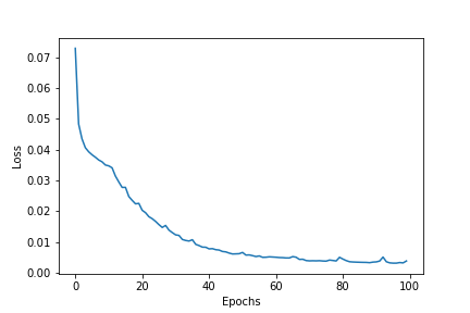
Our model seems to be doing well. Still, we can analyze better if we take a look at the decoded images. The following are some images from training.

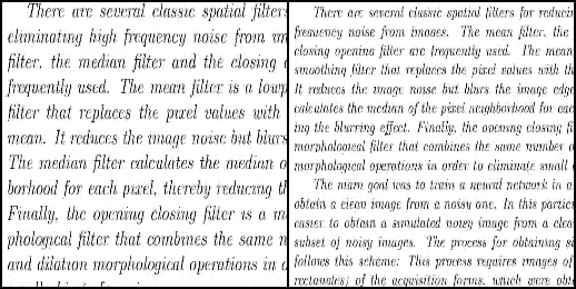
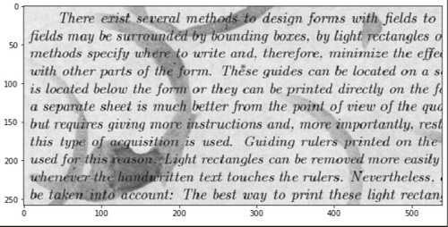
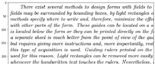
The first image shows the denoised image by the autoencoder at the very beginning of the training. As expected, nothing is readable. The second image shows the denoised image after 90 epochs. We can read almost all the words now and the background noise if completely eliminated.

Now let’s take a look at the test reconstruction images.

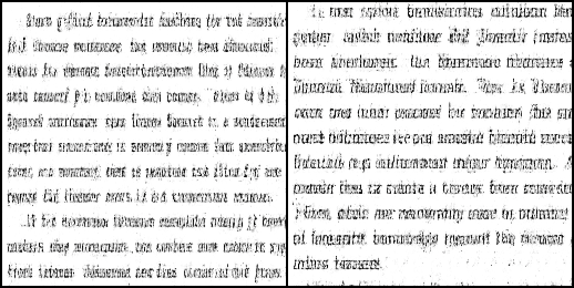
For the test data, we are not getting as good results. The background noise is almost eliminated obviously. But the letters are not much readable. Most probably, the next step to good results might be adding a regularizer to the optimizer. We are not going to cover that in this article. But be sure to post your findings in the comment section if you try it out.

Where to Learn More About Autoencoders

I have written many articles on autoencoder on Debugger Cafe. If you want to learn more, you can surely take a look at the other articles as well. I am sure that they will help you a lot.

Summary and Conclusion

You can contact me using the Contact section. You can also find me on LinkedIn, and Twitter.