Transfer Learning with PyTorch

In deep learning, you will not be writing your custom neural network always. It is almost always better to use transfer learning which gives much better results most of the time. In this article, we will take a look at transfer learning using VGG16 with PyTorch deep learning framework. PyTorch makes it really easy to use transfer learning.

If you are new to PyTorch, then don’t miss out on my previous article series: Deep Learning with PyTorch.

What is Transfer Learning?

Transfer learning is specifically using a neural network that has been pre-trained on a much larger dataset. The main benefit of using transfer learning is that the neural network has already learned many important features from a large dataset. When we use that network on our own dataset, we just need to tweak a few things to achieve good results.

When to Use Transfer Learning?

In deep learning, transfer learning is most beneficial when we cannot obtain a huge dataset to train our network on. In some cases, we may not be able to get our hands on a big enough dataset. For such situations, using a pre-trained network is the best approach. A pre-trained network has already learned many important intermediate features from a larger dataset. Therefore, we can use that network on our small dataset.

What Will We Use in this Article?

In this article, we will use the VGG16 network which uses the weights from the ImageNet dataset.

ImageNet contains more than 14 million images covering almost 22000 categories of images. It has held the ILSVRC (ImageNet Large Scale Visual Recognition Challenge) for years so that deep learning researchers and practitioners can use the huge dataset to come up with novel and sophisticated neural network architectures by using the images for training the networks.

VGG16

We will be downloading the VGG16 from PyTorch models and it uses the weights of ImageNet. The VGG network model was introduced by Karen Simonyan and Andrew Zisserman in the paper named Very Deep Convolutional Networks for Large-Scale Image Recognition. Be sure to give the paper a read if you like to get into the details.

The following is the ConvNet Configuration from the original paper.

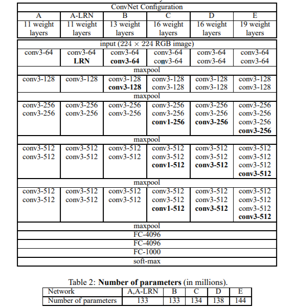
Specifically, we will be using the 16 layer architecture, which is the VGG16 model. VGG16 has 138 million parameters in total.

VGG Network Model Results on ImageNet

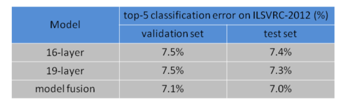
In 2014, VGG models achieved great results in the ILSVRC challenge. The 16 layer model achieved 92.6% top-5 classification accuracy on the test set. Similarly, the 19 layer model was able to achieve 92.7% top-5 accuracy on the test set.

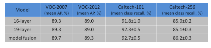
The following images show the VGG results on the ImageNet, PASCAL VOC and Caltech image dataset.

Our Approach

We will use the VGG16 network to classify CIFAR10 images. This is not a very big dataset, but still enough to get started with transfer learning.

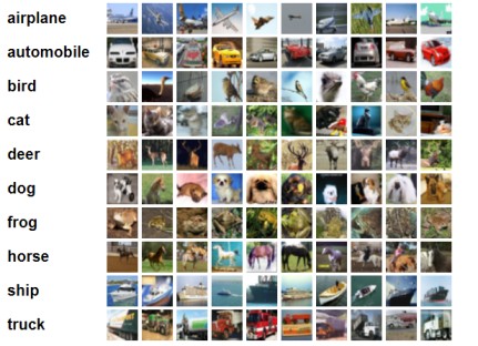
The CIFAR10 dataset contains images belonging to 10 classes. It has 60000 images in total. There are 50000 images for training and 10000 images for testing. All the images are of size 32×32.

Along with the code, we will also analyze the plots for train accuracy & loss and test accuracy & loss as well. This will give us a better perspective on the performance of our network.

So, let’s get started.

Importing Required Modules and Libraries

Here, we will import the required modules that we will need further in the article. These are very standard modules of PyTorch that are used regularly. So, you should not face many difficulties here.

import torch
import torchvision
import torchvision.transforms as transforms
import torch.optim as optim
import time
import torch.nn.functional as F
import torch.nn as nn
import matplotlib.pyplot as plt

from torchvision import models

The models module from torchvision will help us to download the VGG16 neural network.

The next block of code is for checking the CUDA availability. If you have a dedicated CUDA GPU device, then it will be used. Else, further on, your CPU will be used for the neural network operations.

# check GPU availability
device = torch.device("cuda:0" if torch.cuda.is_available() else "cpu")
print(device)

Downloading and Preparing the Dataset

In this section, we will define all the preprocessing operations for the images. Along with that, we will download the CIFAR10 data and convert them using the DataLoader module.

transform = transforms.Compose(
    [transforms.Resize((224, 224)),
     transforms.ToTensor(),
     transforms.Normalize((0.5, 0.5, 0.5), (0.5, 0.5, 0.5))])

trainset = torchvision.datasets.CIFAR10(root='./data', train=True,
                                        download=True, transform=transform)
trainloader = torch.utils.data.DataLoader(trainset, batch_size=32,
                                          shuffle=True)

testset = torchvision.datasets.CIFAR10(root='./data', train=False,
                                       download=True, transform=transform)
testloader = torch.utils.data.DataLoader(testset, batch_size=32,
                                         shuffle=False)

You may observe that one of the transforms is resizing the images to 224×224 size. Well, this is because the VGG network takes an input image of size 224×224 by default. So, it is best to resize the CIFAR10 images as well.

Another thing to take care of here is the batch size. Remember that, if the CUDA device is being used, then we will be loading all the data and the VGG16 model into the CUDA GPU memory. This may require a lot of GPU RAM. If you face OOM (Out Of Memory) error, then consider reducing the batch size. It is best to choose the batch size as a multiple of 2. So, you may choose either 16, 8, or 4 according to your requirement.

Downloading the VGG16 Network

We are now going to download the VGG16 model from PyTorch models. The following code loads the VGG16 model. If you have never run the following code before, then first it will download the VGG16 model onto your system.

vgg16 = models.vgg16(pretrained=True)
vgg16.to(device)

print(vgg16)

At line 1 of the above code block, we load the model. The argument pretrained=True implies to load the ImageNet weights for the pre-trained model. Line 2 loads the model onto the device, that may be the CPU or GPU.

Printing the model will give the following output.

VGG(
  (features): Sequential(
    (0): Conv2d(3, 64, kernel_size=(3, 3), stride=(1, 1), padding=(1, 1))
    (1): ReLU(inplace=True)
    (2): Conv2d(64, 64, kernel_size=(3, 3), stride=(1, 1), padding=(1, 1))
    (3): ReLU(inplace=True)
    (4): MaxPool2d(kernel_size=2, stride=2, padding=0, dilation=1, ceil_mode=False)
    (5): Conv2d(64, 128, kernel_size=(3, 3), stride=(1, 1), padding=(1, 1))
    (6): ReLU(inplace=True)
    (7): Conv2d(128, 128, kernel_size=(3, 3), stride=(1, 1), padding=(1, 1))
    (8): ReLU(inplace=True)
    (9): MaxPool2d(kernel_size=2, stride=2, padding=0, dilation=1, ceil_mode=False)
    (10): Conv2d(128, 256, kernel_size=(3, 3), stride=(1, 1), padding=(1, 1))
    (11): ReLU(inplace=True)
    (12): Conv2d(256, 256, kernel_size=(3, 3), stride=(1, 1), padding=(1, 1))
    (13): ReLU(inplace=True)
    (14): Conv2d(256, 256, kernel_size=(3, 3), stride=(1, 1), padding=(1, 1))
    (15): ReLU(inplace=True)
    (16): MaxPool2d(kernel_size=2, stride=2, padding=0, dilation=1, ceil_mode=False)
    (17): Conv2d(256, 512, kernel_size=(3, 3), stride=(1, 1), padding=(1, 1))
    (18): ReLU(inplace=True)
    (19): Conv2d(512, 512, kernel_size=(3, 3), stride=(1, 1), padding=(1, 1))
    (20): ReLU(inplace=True)
    (21): Conv2d(512, 512, kernel_size=(3, 3), stride=(1, 1), padding=(1, 1))
    (22): ReLU(inplace=True)
    (23): MaxPool2d(kernel_size=2, stride=2, padding=0, dilation=1, ceil_mode=False)
    (24): Conv2d(512, 512, kernel_size=(3, 3), stride=(1, 1), padding=(1, 1))
    (25): ReLU(inplace=True)
    (26): Conv2d(512, 512, kernel_size=(3, 3), stride=(1, 1), padding=(1, 1))
    (27): ReLU(inplace=True)
    (28): Conv2d(512, 512, kernel_size=(3, 3), stride=(1, 1), padding=(1, 1))
    (29): ReLU(inplace=True)
    (30): MaxPool2d(kernel_size=2, stride=2, padding=0, dilation=1, ceil_mode=False)
  )
  (avgpool): AdaptiveAvgPool2d(output_size=(7, 7))
  (classifier): Sequential(
    (0): Linear(in_features=25088, out_features=4096, bias=True)
    (1): ReLU(inplace=True)
    (2): Dropout(p=0.5, inplace=False)
    (3): Linear(in_features=4096, out_features=4096, bias=True)
    (4): ReLU(inplace=True)
    (5): Dropout(p=0.5, inplace=False)
    (6): Linear(in_features=4096, out_features=1000, bias=True)
  )
)

Freezing Convolution Weights

One important thing to notice here is that the classifier model is classifying 1000 classes. You can observe the very last Linear block to confirm that. But we need to classify the images into 10 classes only. So, we will change that. Also, we will freeze all the weights of the convolutional blocks. The model as already learned many features from the ImageNet dataset. So, freezing the Conv2d() weights will make the model to use all those pre-trained weights. This is the part that really justifies the term transfer learning.

The following block of code makes the necessary changes for the 10 class classification along with freezing the weights.

# change the number of classes 
vgg16.classifier[6].out_features = 10

# freeze convolution weights
for param in vgg16.features.parameters():
    param.requires_grad = False

Optimizer and Loss Function

We will use the CrossEntropyLoss() and SGD() optimizer which works quite well in most cases. Let’s define those two and move ahead.

# optimizer
optimizer = optim.SGD(vgg16.classifier.parameters(), lr=0.001, momentum=0.9)
# loss function
criterion = nn.CrossEntropyLoss()

Training and Validation Functions

We will write two different methods here. One is for validation and one for training. Let’s write down the code first, and then get down to the explanation.

# validation function
def validate(model, test_dataloader):
    model.eval()
    val_running_loss = 0.0
    val_running_correct = 0
    for int, data in enumerate(test_dataloader):
        data, target = data[0].to(device), data[1].to(device)
        output = model(data)
        loss = criterion(output, target)
        
        val_running_loss += loss.item()
        _, preds = torch.max(output.data, 1)
        val_running_correct += (preds == target).sum().item()
    
    val_loss = val_running_loss/len(test_dataloader.dataset)
    val_accuracy = 100. * val_running_correct/len(test_dataloader.dataset)
    
    return val_loss, val_accuracy

In the validate() method, we are calculating the loss and accuracy. But we are not backpropagating the gradients. Backpropagation is only required during training.

Next, we will define the fit() method for training.

# training function
def fit(model, train_dataloader):
    model.train()
    train_running_loss = 0.0
    train_running_correct = 0
    for i, data in enumerate(train_dataloader):
        data, target = data[0].to(device), data[1].to(device)
        optimizer.zero_grad()
        output = model(data)
        loss = criterion(output, target)
        train_running_loss += loss.item()
        _, preds = torch.max(output.data, 1)
        train_running_correct += (preds == target).sum().item()
        loss.backward()
        optimizer.step()
    train_loss = train_running_loss/len(train_dataloader.dataset)
    train_accuracy = 100. * train_running_correct/len(train_dataloader.dataset)

    print(f'Train Loss: {train_loss:.4f}, Train Acc: {train_accuracy:.2f}')
    
    return train_loss, train_accuracy

As you can see, at line 14 of the fit() method, we are calculating the gradients and backpropagating.

We will train and validate the model for 10 epochs. All the while, both methods, the fit(), and validate() will keep on returning the loss and accuracy values for each epoch.

Let’s train the model for 10 epochs. For each epoch, we will call the fit() and validate() method.

train_loss , train_accuracy = [], []
val_loss , val_accuracy = [], []
start = time.time()
for epoch in range(10):
    train_epoch_loss, train_epoch_accuracy = fit(vgg16, trainloader)
    val_epoch_loss, val_epoch_accuracy = validate(vgg16, testloader)
    train_loss.append(train_epoch_loss)
    train_accuracy.append(train_epoch_accuracy)
    val_loss.append(val_epoch_loss)
    val_accuracy.append(val_epoch_accuracy)
end = time.time()

print((end-start)/60, 'minutes')

Train Loss: 0.0256, Train Acc: 73.44
Validation Loss: 0.0158, Validation Acc: 82.35
Train Loss: 0.0148, Train Acc: 83.38
Validation Loss: 0.0138, Validation Acc: 84.97
Train Loss: 0.0117, Train Acc: 86.85
Validation Loss: 0.0128, Validation Acc: 86.00
Train Loss: 0.0094, Train Acc: 89.54
Validation Loss: 0.0125, Validation Acc: 86.36
Train Loss: 0.0074, Train Acc: 91.75
Validation Loss: 0.0127, Validation Acc: 86.57
Train Loss: 0.0057, Train Acc: 93.75
Validation Loss: 0.0127, Validation Acc: 86.91
Train Loss: 0.0043, Train Acc: 95.23
Validation Loss: 0.0129, Validation Acc: 86.99
Train Loss: 0.0032, Train Acc: 96.53
Validation Loss: 0.0133, Validation Acc: 87.42
Train Loss: 0.0023, Train Acc: 97.67
Validation Loss: 0.0138, Validation Acc: 87.48
Train Loss: 0.0018, Train Acc: 98.32
Validation Loss: 0.0144, Validation Acc: 87.36

After each epoch, we are saving the training accuracy and loss values in train_accuracy, train_loss and val_accuracy, val_loss. We can see that by the end of the training, our training accuracy is 98.32%.

Visualizing the Plots

Now, let’s visualize the accuracy and loss plots for better clarification.

plt.figure(figsize=(10, 7))
plt.plot(train_accuracy, color='green', label='train accuracy')
plt.plot(val_accuracy, color='blue', label='validataion accuracy')
plt.legend()
plt.savefig('accuracy.png')
plt.show()

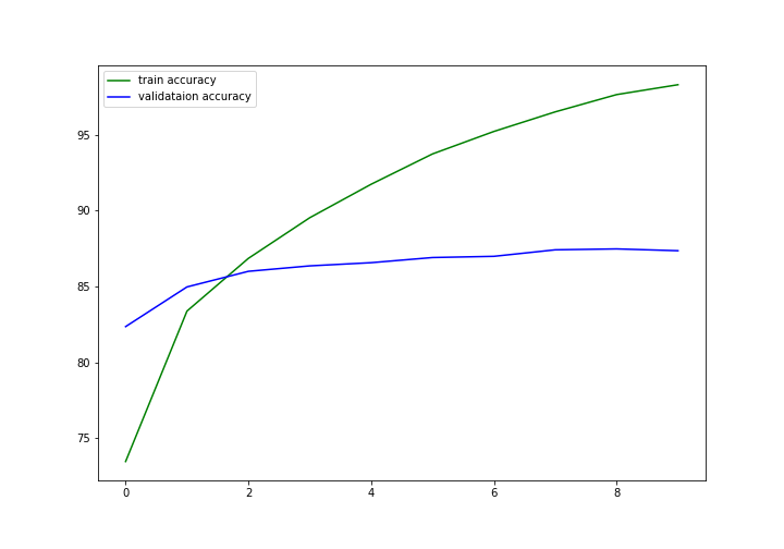
We can see that the validation accuracy was more at the beginning. But with advancing epochs, finally, the model was able to learn the important features. By the end of the training, the training accuracy is much higher than the validation accuracy. Specifically, we are getting about 98% training and 87% validation accuracy.

plt.figure(figsize=(10, 7))
plt.plot(train_loss, color='orange', label='train loss')
plt.plot(val_loss, color='red', label='validataion loss')
plt.legend()
plt.savefig('loss.png')
plt.show()

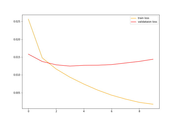
The loss values also follow a similar pattern as the accuracy. First, the validation loss was lower. But eventually, the training loss became much lower than the validation loss.

Summary and Conclusion

We are getting fairly good results, but we can do even better. If you want you can fine-tune the features model values of VGG16 and try to get even more accuracy. One way to get started is to freeze some layers and train some others. We have only tried freezing all of the convolution layers. Be sure to try that out.

I hope that you learned something from this article that you will be able to implement on your own personal projects. You can comment and leave your thoughts and queries in the comment section. I will try my best to address them. If you want, you can contact me on LinkedIn and Twitter.