Creating Efficient Image Data Loaders in PyTorch for Deep Learning

In this tutorial, we will learn how to create efficient data loaders for image data in PyTorch and deep learning. Specifically, this tutorial will help you to handle large image datasets in deep learning. It will also teach you how to use PyTorch DataLoader efficiently for deep learning image recognition.

Introduction and Overview

Working with image data in deep learning can demand a huge amount of memory. And by memory, I mean both, the main memory (RAM), and the GPU memory.

A very common way to handle image data for recognition purposes in deep learning is by creating lists. We read the images from the disk and keep appending the pixel values to the lists. This is a good way but to a certain limit.

And this limit is due to the number of images we have, the size of the images, and the main memory, which is the amount of RAM that we have.

Let’s take a simple example to simulate the above method. Suppose that we are building a cat classifier and we have 20000 cat images saved in the disk. With the above method, the steps will look somewhat like the following:

• read the image paths till we reach 20000 cat images:
  • keep appending the read images to a list, say `image_list`.

After saving all the image pixel values to a list, we may move further to the train-test split and start writing the training code.

Note: Please note that in the above method, we append the pixel values to the list and not the image paths. This is a very important thing to keep in mind.

The above method works well for many cases when we are dealing with small datasets and small image dimensions. In fact, datasets like MNIST, Fashion MNIST, and CIFAR10 are all loaded into the main memory directly. So, what is the problem with the above method?

The Problem with Loading Every Image to Main Memory at the Same Time

When using the above method, it works best when you have either a small dataset or small resolution images. For example, the MNIST and Fashion MNIST images contain 70000 images each in total. All the images are 28×28 in pixel. And the CIFAR10 dataset contains 60000 colored images of 32×32 dimensions. Although the above three datasets contain thousands of images, they are very small resolution images.

But what if we have hundreds of thousands of images of 224×224 each? This is where the real problem starts. Actually, it is possible, but only if you have a lot of RAM at your disposal, like 32 or 64 gigabytes of RAM. And I have seen that 80000 images of 400×400 pixels can easily consume more than 24 gigabytes of RAM.

Now, if you are a professional deep learning researcher or practitioner, then you may have such a beasty system. But frankly, not everyone does. And mainly if you are only experimenting or starting out with deep learning, then it is very unlikely that you have a system with 64 gigabytes of RAM.

The Solution that We Will be Employing

We will use PyTorch deep learning library in this tutorial to learn about creating efficient data loaders. In simple terms, we will load the images into the main memory during training time as batches.

Using batches to load images into the main memory during training time helps us from consuming all of our resources altogether. The best part is that we can use our GPU for training. So, instead of loading the images into RAM, we can load the images to the GPU memory directly.

The Dataset that We Will be Using

Now, many of you may be familiar with the above method of sampling batches of images during training time and loading it into the GPU memory.

But most of the time, the image dataset is coupled with a CSV file with a target column. This target column tells us the class that the image belongs to. What if the dataset contains only images and not the CSV file? For that, we will create our own CSV file indicating a target column.

This tutorial will help you learn how efficiently you can manage image data in deep learning even if it does not come with a CSV file.

The dataset that we are going to use is the Natural Images dataset from Kaggle. This dataset contains 6899 images belonging to 8 distinct classes. The classes are airplane, car, cat, dog, flower, fruit, motorbike and person.

Dataset Distribution

Go ahead and download the dataset. In the next section, we will discuss the project’s directory structure and where to keep what. If you observe, then you will find that the images are saved in their respective class directories.

airplane contains all the images of planes.
cat contains all cat images.
person directory has all images of different persons.
…

Each of the directories contains anywhere between 700 to 1000 images. Now, this is not a very large dataset to check our efficient data loader technique. But this will help us grasp the concepts and we can learn how to code everything using PyTorch. This will help us to work on even larger datasets in the future.

Note: I will be posting an ASL (American Sign Language) recognizer article in one of the future posts. This dataset contains tens of thousands of images where we can test the full potential of efficient data loading during training time. Stay tuned for the upcoming article.

But the dataset does not come with any CSV file to indicate the classes of each image. So, first, we will create our own CSV file. After that, we will also train a ResNet-50 neural network model on the dataset using the efficient data loading technique.

Project Directory Structure

After downloading the Natural Images dataset, you will have a natural-images.zip file.

Before extracting its contents, please do check out the directory structure for this project.

├───input
│   └───natural-images
│       └───natural_images
│           ├───airplane
│           ├───car
│           ├───cat
│           ├───dog
│           ├───flower
│           ├───fruit
│           ├───motorbike
│           └───person
├───outputs
└───src
        create_dataset.py
        test.py
        train.py

• Move the natural-images.zip file to input folder and extract it there. The file will extract as /natural-images/natural_images/ and then it will contain all the directories according to the categories.
• outputs folder will contain the output files that we will save.
• src will contain the python source code files. Basically, we will need three python files. They are create_dataset.py, train.py, and test.py. If you want you can go ahead and creat those python files.

Note: After extracting the zip file, you might find an extra data folder. You can safely ignore or remove that as it is a repetition of the dataset.

Installing Some Important Packages

Before moving further, please make sure that you have the following python packages installed on your system.

Imutils:

Install it by: pip install imutils

Albumentations:

Install it by: pip install albumentations

We will use the albumentations package for fast and efficient image augmentation and transforms during training time.

Okay, now are ready to start writing our code.

Code for Creating Efficient Image Data Loaders in PyTorch

We will start with preparing our dataset so that we can create efficient data loaders.

Preparing the Dataset CSV File

Open up the create_dataset.py file inside the src folder. All of the following code will go into this python file.

This part is going to be very simple, yet very important. This is because we will be creating a CSV file on our own indicating the image paths and their corresponding targets. This will help us to load the images in batches during training time instead of loading all the images into the memory altogether.

Importing the Required Module

Starting with importing all the python modules that we will need for this python code.

import os
import pandas as pd
import numpy as np
import joblib

from imutils import paths
from sklearn.preprocessing import LabelBinarizer
from tqdm import tqdm

Explaining some of the important modules in the above code block.

• We will use LabelBinarizer to binarize all our labels (airplane, car, cat, etc).
• Then joblib will help us to save a pickled (.pkl) version of the binarized labels so that we can load and use that in other code files.

Reading the Image Paths and Preparing the CSV File

In this part, we will read all the image paths and their corresponding categories.

Along with that we will create a CSV file where will will save each of the image paths and the targets.

# get all the image paths
image_paths = list(paths.list_images('../input/natural-images/natural_images'))

# create an empty DataFrame
data = pd.DataFrame()

labels = []
for i, image_path in tqdm(enumerate(image_paths), total=len(image_paths)):
    label = image_path.split(os.path.sep)[-2]
    data.loc[i, 'image_path'] = image_path

    labels.append(label)
    
labels = np.array(labels)
# one hot encode
lb = LabelBinarizer()
labels = lb.fit_transform(labels)

print(f"The first one hot encoded labels: {labels[0]}")
print(f"Mapping an one hot encoded label to its category: {lb.classes_[0]}")
print(f"Total instances: {len(labels)}")

for i in range(len(labels)):
    index = np.argmax(labels[i])
    data.loc[i, 'target'] = int(index)

# shuffle the dataset
data = data.sample(frac=1).reset_index(drop=True)

# save as csv file
data.to_csv('../input/data.csv', index=False)

# pickle the label binarizer
joblib.dump(lb, '../outputs/lb.pkl')
print('Save the one-hot encoded binarized labels as a pickled file.')

print(data.head())

Explaining the Above Code:

• Line 1 gets all the image paths as a list and stores them in image_paths.
• At line 6, we create an empty DataFrame where we will save all the image paths and the labels.
• At line 7, we create an empty list named labels. Then starting from line 8, we read all the image paths and save them under the image_path column in the data DataFrame. Also, at line 12, we append all the labels to the labels list.
• Line 14 converts the labels into an array. Then at line 17, we one-hot encode the labels. After one-hot encoding, for each instance, we will have an array of 8 elements. These 8 elements will correspond to the 8 categories in the dataset. But only the corresponding element will be 1 and all the other 7 will be 0. For example, if the category is airplane, then the one-hot encoded label will be this: [1 0 0 0 0 0 0 0].
• Starting from lines 23 to 25, we save the index positions of the one-hot encoded labels where the element is 1. These will act as our targets while training the neural network.
• After that, we shuffle the DataFrame and save it as data.csv file.
• Finally, we save the one-hot encoded binarized labels as a .pkl file.

You can go ahead and run the python file from within the src folder by typing the following command in the terminal.

python create_dataset.py

After executing the file, you will get the following output.

100%|████████████████████████████████████████████████████████████| 6899/6899 [00:04<00:00, 1665.65it/s]
The first one hot encoded labels: [1 0 0 0 0 0 0 0]
Mapping an one hot encoded label to its category: airplane
Total instances: 6899
Save the one-hot encoded binarized labels as a pickled file.
                                          image_path  target
0  ../input/natural-images/natural_images\car\car...     1.0
1  ../input/natural-images/natural_images\fruit\f...     5.0
2  ../input/natural-images/natural_images\airplan...     0.0
3  ../input/natural-images/natural_images\flower\...     4.0
4  ../input/natural-images/natural_images\fruit\f...     5.0

Writing the Neural Network Training Code

In this section, we will writing the code to train our neural network model. All of the code will go into the train.py file inside the src folder.

We will use The ResNet-50 neural network architecture to train on our dataset. As we do not have a lot of images, therefore, we will use pretrained ImageNet weights.

The training part is going to be very simple and almost like any other PyTorch training code, except a few distinctions. As we already have prepared a CSV file mapping the image paths to the targets, therefore, our work is going to be really easier.

Importing the Required Modules and Libraries

Let’s import all the required libraries and modules first.

import pandas as pd
import joblib
import numpy as np
import torch
import random
import albumentations
import matplotlib.pyplot as plt
import argparse
import torch.nn as nn
import torch.nn.functional as F
import torch.optim as optim
import time

from PIL import Image
from tqdm import tqdm
from torchvision import models as models
from sklearn.model_selection import train_test_split
from torch.utils.data import Dataset, DataLoader

Some of the important utilities are:

• joblib to load the pickled binarized labels.
• albumentations will help us to augment and transform the images.
• We will use argparse to parse the command line arguments. The only command line argument will be the number of epochs.
• PyTorch Dataset and DataLoader to prepare our custom dataset module and the training and testing data loaders.

The next block of code applies a seed to our code for reproducibility and also sets the computation device. The computation device is either the GPU or the CPU.

''' SEED Everything '''
def seed_everything(SEED=42):
    random.seed(SEED)
    np.random.seed(SEED)
    torch.manual_seed(SEED)
    torch.cuda.manual_seed(SEED)
    torch.cuda.manual_seed_all(SEED)
    torch.backends.cudnn.benchmark = True 
SEED=42
seed_everything(SEED=SEED)
''' SEED Everything '''

# set computation device
device = ('cuda:0' if torch.cuda.is_available() else 'cpu')

print(f"Computation device: {device}")

Now, let’s construct the argument parser and parse the arguments. For, the command line arguments, we will be providing only the number of epochs.

# construct the argument parser and parse the arguments
parser = argparse.ArgumentParser()
parser.add_argument('-e', '--epochs', default=10, type=int,
    help='number of epochs to train the model for')
args = vars(parser.parse_args())

We have set the default values for the number of epochs as 10.

Prepare the Dataset and the Data Loaders

Here, we will prepare our dataset.

• First, we will read the CSV file and get the image paths and the corresponding targets.
• We will split the dataset into a train set and a validation set.
• Then we will write the code for the NaturalImageDataset() module.
• Finally, we will prepare the train and test loaders.

Read the CSV File and Divide Into Train and Test Set

Let’s first read the data.csv file.

# read the data.csv file and get the image paths and labels
df = pd.read_csv('../input/data.csv')
X = df.image_path.values
y = df.target.values

In the above code block, we store the image paths and the targets in X and y respectively.

We will use 75% of the data for training and 25% of the data for validation. For splitting the dataset, we will use Scikit-Learn’s train_test_split().

(xtrain, xtest, ytrain, ytest) = (train_test_split(X, y, 
                                test_size=0.25, random_state=42))

Creating the Dataset Module

We will create our own dataset module and call it NaturalImageDataset().

As we only have around 7000 images in our dataset, therefore we will employ image augmentation using the albumentations package. Along with that we will also be using pretrained ResNet-50 model so that we can get better performance on such small dataset.

The following block of code defines the NaturalImageDataset() module.

# image dataset module
class NaturalImageDataset(Dataset):
    def __init__(self, path, labels, tfms=None):
        self.X = path
        self.y = labels

        # apply augmentations
        if tfms == 0: # if validating
            self.aug = albumentations.Compose([
                albumentations.Resize(224, 224, always_apply=True),
                albumentations.Normalize(mean=[0.485, 0.456, 0.406],
                          std=[0.229, 0.224, 0.225], always_apply=True)
            ])
        else: # if training
            self.aug = albumentations.Compose([
                albumentations.Resize(224, 224, always_apply=True),
                albumentations.HorizontalFlip(p=1.0),
                albumentations.ShiftScaleRotate(
                    shift_limit=0.3,
                    scale_limit=0.3,
                    rotate_limit=30,
                    p=1.0
                ),
                albumentations.Normalize(mean=[0.485, 0.456, 0.406],
                          std=[0.229, 0.224, 0.225], always_apply=True)
            ])

    def __len__(self):
        return (len(self.X))
    
    def __getitem__(self, i):
        image = Image.open(self.X[i])
        image = self.aug(image=np.array(image))['image']
        image = np.transpose(image, (2, 0, 1)).astype(np.float32)
        label = self.y[i]

        return torch.tensor(image, dtype=torch.float), torch.tensor(label, dtype=torch.long)

• Starting from line 3, first we have our __init__() function where we initialize the image paths and the labels.
• Then we define two sets of image augmentation, one for validation and the other one for training.
  • While validating, we are only resizing and normalizing the images.
  • For training, we are employing a bit more extensive set of image augmentations. We are horizontally flipping the images. Along with that, we are shifting, scaling, and rotating the images as well.
• From line 31, we define the __getitem__() function.
  • First, we open the image by reading it according to the path.
  • At line 33, we apply the image augmentations.
  • Then we transpose the image dimensions so that we can get channels first, then the height, and then the width (c, h, w).
  • Line 35 get the label of the image.
  • Finally, at line 37, we return the image and the labels as tensors.

Creating the Iterable Data Loaders

First, we will create the train_data and test_data, and then we will create the iterable data loader.

train_data = NaturalImageDataset(xtrain, ytrain, tfms=1)
test_data = NaturalImageDataset(xtest, ytest, tfms=0)
 
# dataloaders
trainloader = DataLoader(train_data, batch_size=32, shuffle=True)
testloader = DataLoader(test_data, batch_size=32, shuffle=False)

Both, the trainloader and the testloader have a batch size of 32. We are shuffling the trainloader only, and not the testloader.

Loading the Binarized Labels and Preparing the Neural Network Model

We can load the binarized labels that we have saved before. This is important because the length of the binarized labels file, that is, the length of lb.pkl gives the number of classes in our dataset.

We need the number of classes to fine-tune the final classification layer of the ResNet-50 model. Although we know that there are 8 classes, still it is not a very good idea to hardcode it.

The following block of code loads the binarized labels file.

# load the binarized labels
print('Loading label binarizer...')
lb = joblib.load('../outputs/lb.pkl')

Defining the ResNet-50 Model

Now, we can define the ResNet-50 model.

def model(pretrained, requires_grad):
    model = models.resnet50(progress=True, pretrained=pretrained)
    # freeze hidden layers
    if requires_grad == False:
        for param in model.parameters():
            param.requires_grad = False
    # train the hidden layers
    elif requires_grad == True:
        for param in model.parameters():
            param.requires_grad = True
    # make the classification layer learnable
    model.fc = nn.Linear(2048, len(lb.classes_))
    return model
model = model(pretrained=True, requires_grad=False).to(device)
print(model)

We are loading the ResNet-50 model with the ImageNet weights. Also, note that we are freezing the hidden layers. This will prevent from backpropagating the gradients of the hidden layers so that those weights do not change while training. Finally, we are fine-tuning the last classification layer of the ResNet-50 model (line 12).

Note that for the number of classes we have give the length of the binarized labels file as we have discussed above.

We also need to define the optimizer and the criterion for our neural network model. We will use the SGD optimizer with the learning rate of 0.0001 and weight decay of 0.0005. For the criterion, we will use the CrossEntropyLoss().

# optimizer
optimizer = optim.SGD(model.parameters(), lr=1e-4, momentum=0.9, weight_decay=0.0005)
# loss function
criterion = nn.CrossEntropyLoss()

The Validation and Training Functions

If you have been coding in PyTorch for some time, then you will find this section very familiar. We will define very simple validation and training functions.

In each of the function, we will return the loss and accuracy epoch-wise.

The Validation Function

First, let’s define the validation function. We will be calling it validate().

#validation function
def validate(model, test_dataloader):
    print('Validating')
    model.eval()
    val_running_loss = 0.0
    val_running_correct = 0
    with torch.no_grad():
        for i, data in tqdm(enumerate(test_dataloader), total=int(len(test_data)/test_dataloader.batch_size)):
            data, target = data[0].to(device), data[1].to(device)
            outputs = model(data)
            loss = criterion(outputs, target)
            
            val_running_loss += loss.item()
            _, preds = torch.max(outputs.data, 1)
            val_running_correct += (preds == target).sum().item()
        
        val_loss = val_running_loss/len(test_dataloader.dataset)
        val_accuracy = 100. * val_running_correct/len(test_dataloader.dataset)
        print(f'Val Loss: {val_loss:.4f}, Val Acc: {val_accuracy:.2f}')
        
        return val_loss, val_accuracy

Observe that we are not backpropagating the gradients or updating the parameters. We do not need those during validation on the dataset. Also, the validation code is within a with torch.no_grad(). This prevents the gradients from being calculated during validation.

The Training Function

We call the training function as fit() and the following code block defines it.

# training function
def fit(model, train_dataloader):
    print('Training')
    model.train()
    train_running_loss = 0.0
    train_running_correct = 0
    for i, data in tqdm(enumerate(train_dataloader), total=int(len(train_data)/train_dataloader.batch_size)):
        data, target = data[0].to(device), data[1].to(device)
        optimizer.zero_grad()
        outputs = model(data)
        loss = criterion(outputs, target)
        train_running_loss += loss.item()
        _, preds = torch.max(outputs.data, 1)
        train_running_correct += (preds == target).sum().item()
        loss.backward()
        optimizer.step()
        
    train_loss = train_running_loss/len(train_dataloader.dataset)
    train_accuracy = 100. * train_running_correct/len(train_dataloader.dataset)
    
    print(f"Train Loss: {train_loss:.4f}, Train Acc: {train_accuracy:.2f}")
    
    return train_loss, train_accuracy

During training, we need to backpropagate the gradients so that the model can learn. We are doing that at line 15. Also, at line 16, we are updating the model parameters. As usual, we are returning train loss and accuracy after each epoch.

Executing the Training and Validation Functions

We will run the fit() and validate() function for the number epochs as specified in the command line while executing the train.py file.

train_loss , train_accuracy = [], []
val_loss , val_accuracy = [], []
start = time.time()
for epoch in range(args['epochs']):
    print(f"Epoch {epoch+1} of {args['epochs']}")
    train_epoch_loss, train_epoch_accuracy = fit(model, trainloader)
    val_epoch_loss, val_epoch_accuracy = validate(model, testloader)
    train_loss.append(train_epoch_loss)
    train_accuracy.append(train_epoch_accuracy)
    val_loss.append(val_epoch_loss)
    val_accuracy.append(val_epoch_accuracy)
end = time.time()

print(f"{(end-start)/60:.3f} minutes")

After each epoch, we are appending the loss and accuracy values to lists. For the fit() function, we are storing the values in train_loss and train_accuracy. And for the validation() function, we are storing them in val_loss and val_accuracy.

Now, we need to save the loss and accuracy plots to disk. This will help us to analyze them later.

# accuracy plots
plt.figure(figsize=(10, 7))
plt.plot(train_accuracy, color='green', label='train accuracy')
plt.plot(val_accuracy, color='blue', label='validataion accuracy')
plt.xlabel('Epochs')
plt.ylabel('Accuracy')
plt.legend()
plt.savefig('../outputs/accuracy.png')
plt.show()

# loss plots
plt.figure(figsize=(10, 7))
plt.plot(train_loss, color='orange', label='train loss')
plt.plot(val_loss, color='red', label='validataion loss')
plt.xlabel('Epochs')
plt.ylabel('Loss')
plt.legend()
plt.savefig('../outputs/loss.png')
plt.show()

Finally, we just need to save the trained model to disk. We will be testing our trained model on unseen data, therefore, it is important to save it. The following block of code saves the model.

# save the model to disk
print('Saving model...')
torch.save(model.state_dict(), '../outputs/model.pth')

Executing our train.py File

The final step of training our ResNet-50 deep neural network model is executing the train.py file. Type the following command while still being within the src folder.

python train.py --epochs 10

So, we are training our neural network model for 10 epcohs.

Let’s take a look some of the outputs.

Epoch 1 of 10
Training
162it [02:18,  1.17it/s]
Train Loss: 0.0481, Train Acc: 68.42
Validating
54it [01:20,  1.49s/it]
Val Loss: 0.0289, Val Acc: 97.91
Epoch 2 of 10
Training
162it [01:00,  2.66it/s]
Train Loss: 0.0251, Train Acc: 96.23
Validating
54it [00:18,  2.99it/s]
Val Loss: 0.0146, Val Acc: 98.96
...
Epoch 10 of 10
Training
162it [00:43,  3.75it/s]
Train Loss: 0.0053, Train Acc: 98.65
Validating
54it [00:11,  4.56it/s]
Val Loss: 0.0028, Val Acc: 99.42
13.085 minutes
Saving model...

Analyzing the Results

Now, let’s take a look at the accuracy and loss plots for better analysis.

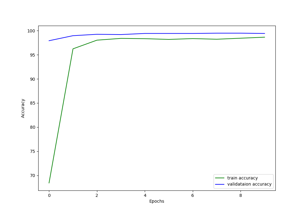
We can see that the validation accuracy is constantly higher than the training accuracy until the end of the training. This is most likely because the model gets to see very less number of validation examples which it finds extremely easy to classify. And due to the data augmentation, the ResNet-50 neural network model finds the training examples just a bit more difficult.

Now, let’s take a look at the loss plot as well.

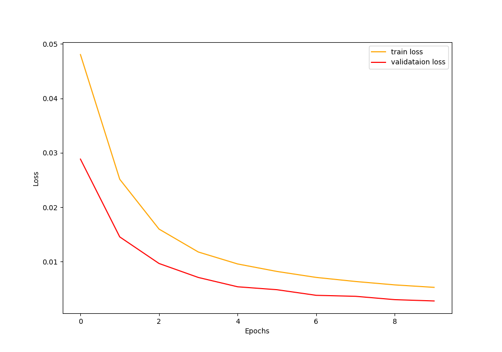
The loss plot also follows a similar pattern where the validation loss is lower than the training loss.

Training for more epochs is also not going to help as the model will surely overfit on such a small dataset. In fact, the ResNet-50 neural network model is an overkill for this dataset containing only around 7000 images. Now, there are some downsides to the results that we are getting. Most probably, the classification result for some images is going to be wrong during testing. In fact, it does, which we will see next.

Then let’s see which images the trained model can classify correctly, and which ones it classifies incorrectly.

Testing Our Trained Neural Network Model

Before moving further, you need to download some images that we will test our model on. Download the following zip file containing three images, a cat, dog, and an airplane image.

After downloading the file, extract its content into the input folder. You should have three images now, cat.jpg, dog.jpg, and plane.jpg.

Okay, now we need to write our test code. All the test code will go into the test.py file.

Writing Our Test Code

It is going to be a very simple code file. The steps are:

• We will load the trained ResNet-50 model.
• Then we will read the image from the path given in the command line argument.
• Give the image to the model to predict its class.
• Use OpenCV to display the image and its class on the image itself.

Importing the Modules

Let’s start with importing the modules.

import torch
import joblib
import torch.nn as nn
import numpy as np
import cv2 as cv
import argparse

from torchvision import models

Argument Parser to Read the Image from the Path

# construct the argument parser and parse the arguments
parser = argparse.ArgumentParser()
parser.add_argument('-i', '--img', default='cat.jpg', type=str,
    help='path for the image to test on')
args = vars(parser.parse_args())

We have given cat.jpg as the default image, in case, we do not specify any image.

Load the Binarized Labels and the Model

First, let’s load the binarized labels. This is required to map the output class to the actual category of the image.

# load label binarizer
lb = joblib.load('../outputs/lb.pkl')

Now, loading the trained ResNet-50 model.

'''MODEL'''
def model(pretrained, requires_grad):
    model = models.resnet50(progress=True, pretrained=pretrained)
    # freeze hidden layers
    if requires_grad == False:
        for param in model.parameters():
            param.requires_grad = False
    # train the hidden layers
    elif requires_grad == True:
        for param in model.parameters():
            param.requires_grad = True
    # make the classification layers learnable
    model.fc = nn.Linear(2048, len(lb.classes_))
    return model
model = model(pretrained=False, requires_grad=False).cuda()
model.load_state_dict(torch.load('../outputs/model.pth'))
print('Model loaded')

Reading the Image and Predicting the Output

This is the final step. Here, we will read the image and predict what our neural network model sees.

image = cv.imread(f"../input/test_images/{args['img']}")
image_copy = image.copy()

image = np.transpose(image, (2, 0, 1)).astype(np.float32)
image = torch.tensor(image, dtype=torch.float).cuda()
image = image.unsqueeze(0)
print(image.shape)

outputs = model(image)
_, preds = torch.max(outputs.data, 1)
print(f"Predicted output: {lb.classes_[preds]}")

cv.putText(image_copy, lb.classes_[preds], (10, 30), cv.FONT_HERSHEY_SIMPLEX, 0.9, (0, 0, 255), 2)
cv.imshow('image', image_copy)
cv.imwrite(f"../outputs/{args['img']}.jpg", image_copy)
cv.waitKey(0)

First, we read the image. Then we also create a copy so that we can display the output on the copied image. After that, we transpose the image dimensions, convert it into PyTorch tensor and predict (line 9) its class.

From lines 13 to 16, we get the predicted class’s actual category name by mapping it using the binarized labels. Then we show the image and the predicted category using OpenCV imshow() function. We also save the image at line 15.

Executing the test.py file

Now, let’s execute the test.py file and see the outputs. We will first test our model on the cat image.

python test.py --img cat.jpg

The following image is shown after execution.

Our trained model is correctly classifying the cat image. Looks like our model has learned after all.

Let’a test on a couple of more images.

python test.py --img dog.jpg

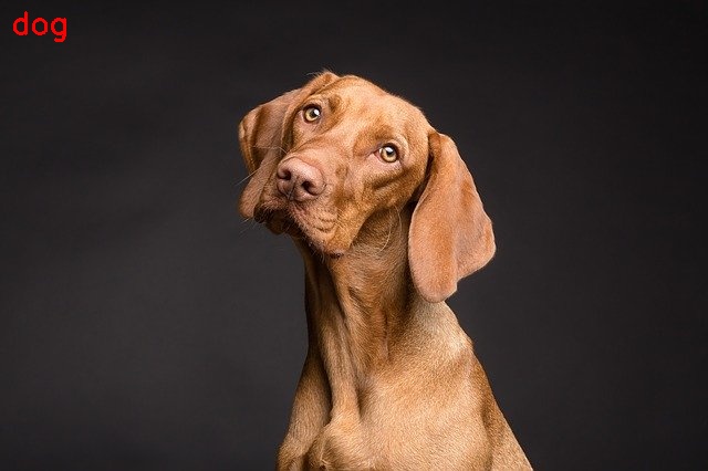
python test.py --img plane.jpg

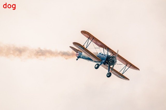
For some reason, our model is classifying the airplane image as a dog. This is probably because our model is overfitting on the validation set and there is a variance between our validation and test images.

This problem perhaps can be solved by getting more images, so that we can train as well as validate on a variety of images. Another important step to consider is to use a smaller neural network architecture and train for longer period.

Summary and Conclusion

In this tutorial you learned:

• How to build memory efficient image data loaders to train deep neural networks.
• Use efficient data loaders to train a ResNet-50 neural network model on Natural Images dataset.

In one of the future posts, we will be working on the ASL (American Sign Language) dataset where we can fully utilize this efficient data loader method. So, stay tuned.

You can leave you thought in the comment section, and I will try my best to address them.

You can contact me using the Contact section. You can also find me on LinkedIn, and Twitter.