Dataset Expansion Using Image Augmentation for Deep Learning

Deep learning algorithms and neural networks work best when we have a huge amount of data. In the case of image recognition, the neural network model always benefits from a large amount of image data. But what if we do not have a large amount of image data for our deep learning algorithm? If you are a deep learning practitioner, then the obvious answer is image augmentation. But there is a catch to using image augmentation in its regular form in deep learning. In this article, we will discuss the issue and also learn how to do dataset expansion using image augmentation.

What will we cover in this article?

• Why do deep learning algorithms require a huge amount of data?
• Why train time image augmentation is useful, but not very effective?
• How we can expand the dataset using image augmentation? And why does it help?
• Training a ResNet18 deep learning model on chess images dataset.

On a side note (yet a really important one), I am really glad to say that DebuggerCafe has been recognized as one of the top 10 deep learning blogs by Feedspot. This is only possible due to the audience that supports me and values my content. This really helps me remain motivated and create the best content possible.

Deep Learning and Dataset Size

We already know very well the importance of huge amounts of data for training deep learning neural networks. The bigger the deep learning architecture, the more data we need. All of these requirements boil down to the number of parameters in a deep learning architecture.

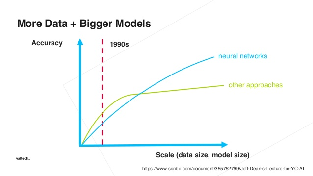
The more the number of parameters to train, the more data we need. Else, the mode will overfit really easily. And we don’t want that.

One of the easier solutions to this problem is using transfer learning. In transfer learning, we can take a neural network model that has been previously trained on a huge dataset similar to the data that we have. Then use that model and fine-tune the classification layers to learn using the new data. And most commonly, we use models that are pre-trained on the huge ImageNet dataset.

But in this case, too, we need at least some thousands of images for a well-trained model that can generalize well.

So, what if we have the images in hundreds and not in thousands? Here, the first step to consider is obviously transfer learning. But still, hundreds of images are too less. One of the other solutions here is image augmentation in deep learning.

Train Time Image Augmentation in Deep Learning

There is another very common and important step that we can take when we have less amount of image data. That is train time image augmentation.

Most of the deep learning frameworks have predefined modules that we can use to augment image data before training the deep learning model.

Nowadays, there are even specific libraries just for augmenting images. Though these libraries perform many other image processing tasks as well.

The Problem with Train Time Image Augmentation

Augmenting the images just before training is one of the most common approaches.

Train time image augmentation works well but there is a catch to it. The image dataset actually does not expand. Rather the augmented images replace the original images. And then these augmented images are used for training. So, our neural network model does not train on more number of images. It trains on the same number of images. It’s just that each of the images is augmented. Depending on the augmentation methods used, the images may be scaled, shifted, or flipped. Instead of the original images, these augmented (but same amount) of images are used for training.

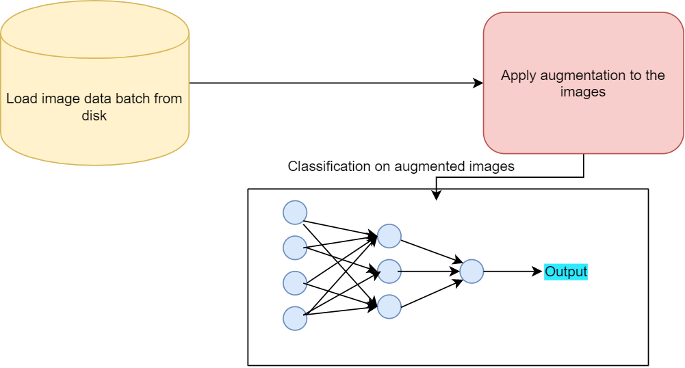
Now, augmenting the images brings some variety to the dataset and the neural network model gets to see different types of those images. This helps as it increases the generalization power of the neural network model.

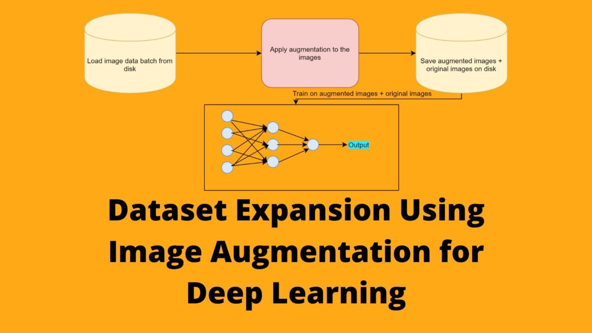
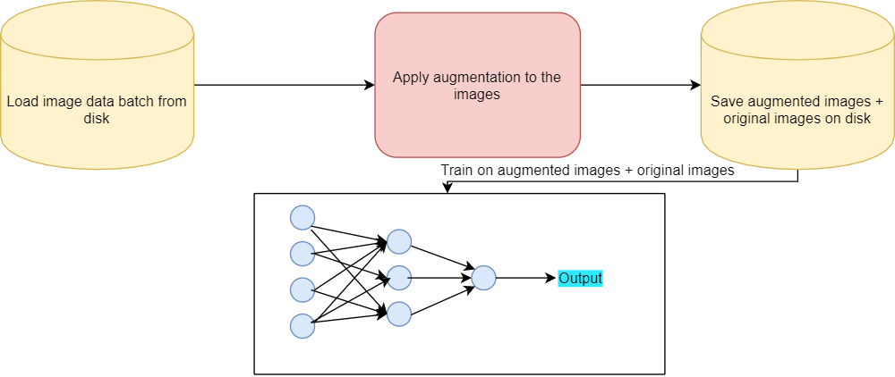
Dataset Expansion using Image Augmentation

One of the other, less used, yet highly effective methods is expansion of the image dataset using image augmentation.

In this method, we use the original images as well as the augmented images for training. So, while training the neural network model will get to see the original images and the augmented images. Using this method, we can increase the size of the image dataset substantially.

Also, when used correctly, each image can be made to look very different from the original images. Using a combination of flipping, scaling, rotating, and shifting usually yields the best results.

In the rest of the tutorial, we will learn how we can use image augmentation to create new images and save them to disk. Then we will use these images as well as the original images to train a ResNet-18 neural network model.

Dataset Expansion Using Image Augmentation and Training a ResNet-18 Model

Beginning from this section, we will take the practical approach to dataset expansion using image augmentation. The following are the steps that we will cover:

• Train a ResNet-18 model on the Chessman Image Dataset from Kaggle using train time image augmentation.
• Analyze the training and validation performance.
• Expand the dataset using image augmentation.
• Again train a ResNet-18 model on the dataset. This time using both, the original images and the augmented images.
• Analyze the training and validation performance.

But first, we need the dataset.

Get the Dataset That We Will Use

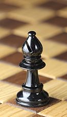
We will use the Chessman image dataset from Kaggle. This dataset contains images of different chess pieces according to the sub-folders. The dataset will download as chessman-image-dataset.zip file. This dataset contains the images of bishop, king, knight, pawn, queen, and rook chess pieces according to the piece type in different subfolders.

For example, Bishop folder contains all the images of bishop chess pieces, King folder all the king chess pieces, and so on. Note that the dataset only contains 551 images in its current form. So, it is going to be a good test for our dataset expansion method.

If you explore the dataset, then you will find that the images have different extensions, ranging from .png to .gif. Also, many are stock photos containing watermarks. Therefore, our recognition model is going to find it a lot difficult in classifying the images.

In the next section, we will see how to structure our directory for this project.

The Directory Structure

The following is the directory structure for our project.

├───input
│   └───chessman-image-dataset
│       └───Chess
│           ├───Bishop
│           ├───King
│           ├───Knight
│           ├───Pawn
│           ├───Queen
│           └───Rook
├───outputs
└───src
        create_aug_images.py
        create_csv.py
        test.py
        train.py

• input folder contains the chessman-image-dataset folder. You will get this after you extract the zip file. Inside that we have Chess folder. It contains all the subfolders according to the chess pieces’ names. These subfolders contain the images.
• Then we have outputs where we will save the accuracy/loss plots and our model after training.
• src folder contains all the python files. We will get to the usage of each python file when we will start the write the code.

Before moving further you need to install the imutils and albumentations package if you do not already have it.

pip install imutils

pip install albumentations

Also, we will use the PyTorch deep learning framework in this tutorial.

Creating a CSV File Mapping the Image Paths to the Targets

In this section, we will create a CSV file mapping the image to the targets. And in our case, our targets are going to be the chess piece categories like the bishop, rook, king, etc.

The following is the code that creates the CSV file as well as the binarized labels for each category. All of this code goes into the create_csv.py file.

import pandas as pd
import numpy as np
import os
import joblib

from sklearn.preprocessing import LabelBinarizer
from tqdm import tqdm
from imutils import paths

# get all the image paths
image_paths = list(paths.list_images('../input/chessman-image-dataset/Chess'))

# create a DataFrame 
data = pd.DataFrame()

labels = []
for i, image_path in tqdm(enumerate(image_paths), total=len(image_paths)):
    label = image_path.split(os.path.sep)[-2]
    # save the relative path for mapping image to target
    data.loc[i, 'image_path'] = image_path

    labels.append(label)

labels = np.array(labels)
# one hot encode the labels
lb = LabelBinarizer()
labels = lb.fit_transform(labels)

print(f"The first one hot encoded labels: {labels[0]}")
print(f"Mapping the first one hot encoded label to its category: {lb.classes_[0]}")
print(f"Total instances: {len(labels)}")

for i in range(len(labels)):
    index = np.argmax(labels[i])
    data.loc[i, 'target'] = int(index)

# shuffle the dataset
data = data.sample(frac=1).reset_index(drop=True)

# save as CSV file
data.to_csv('../input/data.csv', index=False)

# pickle the binarized labels
print('Saving the binarized labels as pickled file')
joblib.dump(lb, '../outputs/lb.pkl')

print(data.head(5))

We save the binarized labels as lb.pkl. We can load this file from the disk whenever we want. The length of this file gives the total number of classes we have. So, we can use this when we will be fine-tuning the classification layer of the ResNet-18 model.

We will not go into the details of this code. You can find the explanation of creating such CSV files and binarized files in much detail in this article. You will get to learn how to create efficient data loaders for image datasets in PyTorch.

Note: I have deliberately skipped the explanation of the above code in this tutorial. Explaining it here will unnecessarily increase the length of the post. Instead you can find all the details in the article mentioned.

Before, moving further, we need to execute the create_csv.py file. Execute it while being in the src folder.

python create_csv.py file

You should see the following output.

100%|██████████████████████████████████████████████████████████████| 551/551 [00:00<00:00, 1854.14it/s]
   The first one hot encoded labels: [1 0 0 0 0 0]
   Mapping the first one hot encoded label to its category: Bishop
   Total instances: 551
...

You can see that there are only 551 images in total. These many images are a very small amount for a neural network to learn anything useful.

After executing the code, you will have a data.csv file inside the input folder. Also, the lb.pkl folder will get created in the outputs folder.

Writing the Training Code for Our Chess Dataset Expansion Using Image Augmentation

Here, we will start to write the code into the train.py file. After writing this code, we can use this for train time augmentation training as well as using both the original images and augmentated images.

Let’s begin with the code implementation.

Importing the Modules

Let’s import all the required modules first.

'''
USAGE:
python train.py --epochs 50
'''

import pandas as pd
import joblib
import numpy as np
import torch
import random
import albumentations
import matplotlib.pyplot as plt
import argparse
import torch.nn as nn
import torch.nn.functional as F
import torch.optim as optim
import time

from PIL import Image
from tqdm import tqdm
from torchvision import models as models
from sklearn.model_selection import train_test_split
from torch.utils.data import Dataset, DataLoader

After importing all the packages and modules, we need to create an argument parser. We will be providing the number of epochs as the command line argument, so we need an argument parser for that.

# construct the argument parser and parse the arguments
parser = argparse.ArgumentParser()
parser.add_argument('-e', '--epochs', default=50, type=int,
    help='number of epochs to train the model for')
args = vars(parser.parse_args())

After that we need to set the seed for reproducibility for multiple runs.

''' SEED Everything '''
def seed_everything(SEED=42):
    random.seed(SEED)
    np.random.seed(SEED)
    torch.manual_seed(SEED)
    torch.cuda.manual_seed(SEED)
    torch.cuda.manual_seed_all(SEED)
    torch.backends.cudnn.benchmark = True 
SEED=42
seed_everything(SEED=SEED)
''' SEED Everything '''

# set computation device
device = ('cuda:0' if torch.cuda.is_available() else 'cpu')

print(f"Computation device: {device}")

In the above code block, we are also setting the computation device at line 14.

Diving the Data into Training and Validation Set

We will divide the whole data into a training and a validation set. We will use 25% of the total data for validation, and the rest, that is, 75% of the data for training.

# read the data.csv file and get the image paths and labels
df = pd.read_csv('../input/data.csv')
X = df.image_path.values
y = df.target.values

(xtrain, xtest, ytrain, ytest) = (train_test_split(X, y, 
                                test_size=0.25, random_state=42))

print(f"Training on {len(xtrain)} images")
print(f"Validationg on {len(xtest)} images")

• At line 2, we read the data.csv file. Then we get the path names and corresponding targets and store them in X and y respectively.
• After that we split the data into training and validation set (line 6).

Creating the Custom Dataset Module and the Data Loaders

We will write our custom dataset module that will fetch the images from the respective image folders. The name of the dataset module is going be ChessImageDataset().

PyTorch provides a very easy and intuitive way to create custom dataset modules. We need to subclass PyTorch Dataset module to do it.

Let’s write the code first, then we will get to the explanation part.

# image dataset module
class ChessImageDataset(Dataset):
    def __init__(self, path, labels, tfms=None):
        self.X = path
        self.y = labels

        # apply augmentations
        if tfms == 0: # if validating
            self.aug = albumentations.Compose([
                albumentations.Resize(224, 224, always_apply=True),
                albumentations.Normalize(mean=[0.485, 0.456, 0.406],
                          std=[0.229, 0.224, 0.225], always_apply=True)
            ])
        else: # if training
            self.aug = albumentations.Compose([
                albumentations.Resize(224, 224, always_apply=True),
                albumentations.HorizontalFlip(p=1.0),
                albumentations.ShiftScaleRotate(
                    shift_limit=0.3,
                    scale_limit=0.3,
                    rotate_limit=30,
                    p=1.0
                ),
                albumentations.Normalize(mean=[0.485, 0.456, 0.406],
                          std=[0.229, 0.224, 0.225], always_apply=True)
            ])

    def __len__(self):
        return (len(self.X))
    
    def __getitem__(self, i):
        image = Image.open(self.X[i])
        image = self.aug(image=np.array(image))['image']
        image = np.transpose(image, (2, 0, 1)).astype(np.float32)
        label = self.y[i]

        return torch.tensor(image, dtype=torch.float), torch.tensor(label, dtype=torch.long)

• In the __init__() method, we are defining the image augmentations using the albumentations library.
  • For the validation set, we will only apply resizing and normalization to the images.
  • For the training set, we will apply horizontal flipping, shifting, scaling, and rotating of the images.
• Starting from line 31, we implement the __getitem__() method. We read each of the images, apply the augmentations, and return the images along with the corresponding labels.

Next up, we will create the trainloader and testloader.

train_data = ChessImageDataset(xtrain, ytrain, tfms=1)
test_data = ChessImageDataset(xtest, ytest, tfms=0)
 
# dataloaders
trainloader = DataLoader(train_data, batch_size=32, shuffle=True)
testloader = DataLoader(test_data, batch_size=32, shuffle=False)

• At line 1 and 2, we get the train_data and test_data. Notice that we are applying the augmentations to the train_data only.
• Then at lines 5 and 6, we are defining the iterable trainloader and testloader that we will use during training and validation.
  • Both of the data loaders have a batch size of 32. We are only shuffling the trainloader and not the testloader.

Load the Binarized Labels and Define the ResNet-18 Neural Network Model

Now, we will load the binarized labels. We need those to fine-tune the classification layer of the ResNet-18 neural network model. The length of the binarized labels’ file gives the number of classes that we have. Although, we can hard code the number of classes as 6, still it is better not to do.

Let’s load those binarized labels.

# load the binarized labels
print('Loading label binarizer...')
lb = joblib.load('../outputs/lb.pkl')

We will use the models module of the PyTorch library to load the ResNet-18 model.

def model(pretrained, requires_grad):
    model = models.resnet18(progress=True, pretrained=pretrained)
    # freeze hidden layers
    if requires_grad == False:
        for param in model.parameters():
            param.requires_grad = False
    # train the hidden layers
    elif requires_grad == True:
        for param in model.parameters():
            param.requires_grad = True
    # make the classification layer learnable
    model.fc = nn.Linear(512, len(lb.classes_))
    return model
model = model(pretrained=True, requires_grad=False).to(device)

We are calling the model() function at line 14. We are giving the arguments pretrained=True, and requires_grad=False. These will load the ImageNet weights into the model for us and freeze the hidden layer weights as well.

Notice that at line 12, we are only making the final classification layer learnable. If you want, you can also add more layers to the head. But for this simple dataset, we will stick with this.

We need to define the optimizer and the loss function for our model as well. For the loss function, we will use CrossEntropyLoss, and for the optimizer, we will use the SGD optimizer.

# optimizer
optimizer = optim.SGD(model.parameters(), lr=1e-3, momentum=0.9, weight_decay=0.0005)
# loss function
criterion = nn.CrossEntropyLoss()

For the SGD optimizer, we are using a learning rate of 0.001 with momentum of 0.9 and weight decay of 0.0005.

The Validation Function

We will define a function called validate() for carrying out the validation. The validate() function takes in two arguments. One is the neural network model and the other is the dataloader. While calling the validate() function we will provide the testloader as the argument for the dataloader parameter.

The following block of code defines the validate() function.

#validation function
def validate(model, dataloader):
    print('Validating')
    model.eval()
    running_loss = 0.0
    running_correct = 0
    with torch.no_grad():
        for i, data in tqdm(enumerate(dataloader), total=int(len(test_data)/dataloader.batch_size)):
            data, target = data[0].to(device), data[1].to(device)
            outputs = model(data)
            loss = criterion(outputs, target)
            
            running_loss += loss.item()
            _, preds = torch.max(outputs.data, 1)
            running_correct += (preds == target).sum().item()
        
        val_loss = running_loss/len(dataloader.dataset)
        val_accuracy = 100. * running_correct/len(dataloader.dataset)
        print(f'Val Loss: {val_loss:.4f}, Val Acc: {val_accuracy:.2f}')
        
        return val_loss, val_accuracy

• We use running_loss and running_correct to keep track of the loss and accuracy for each batch.
• val_loss and val_accuracy define the loss and accuracy for each epoch.
• We are returning the per epoch loss and accuracy at line 21.
• Also, the whole of the validation operation is within the with torch.no_grad() block so as to prevent the calculation of gradients.

The Training Function

The training function (fit()) is very similar to the validation function with a few minor but important changes.

# training function
def fit(model, dataloader):
    print('Training')
    model.train()
    running_loss = 0.0
    running_correct = 0
    for i, data in tqdm(enumerate(dataloader), total=int(len(train_data)/dataloader.batch_size)):
        data, target = data[0].to(device), data[1].to(device)
        optimizer.zero_grad()
        outputs = model(data)
        loss = criterion(outputs, target)
        running_loss += loss.item()
        _, preds = torch.max(outputs.data, 1)
        running_correct += (preds == target).sum().item()
        loss.backward()
        optimizer.step()
        
    train_loss = running_loss/len(dataloader.dataset)
    train_accuracy = 100. * running_correct/len(dataloader.dataset)
    
    print(f"Train Loss: {train_loss:.4f}, Train Acc: {train_accuracy:.2f}")
    
    return train_loss, train_accuracy

• At line 9, we zero out the gradients for the current batch.
• Line 15, backpropagates the gradients.
• Line 16, updates the parameters in the neural network model.

Executing the fit() and validate() Functions

We will train the model for the number of epochs as provided in the command line when executing the train.py file.

The following block of code runs the fit() and validate() function for the specified number of epochs.

train_loss , train_accuracy = [], []
val_loss , val_accuracy = [], []
start = time.time()
for epoch in range(args['epochs']):
    print(f"Epoch {epoch+1} of {args['epochs']}")
    train_epoch_loss, train_epoch_accuracy = fit(model, trainloader)
    val_epoch_loss, val_epoch_accuracy = validate(model, testloader)
    train_loss.append(train_epoch_loss)
    train_accuracy.append(train_epoch_accuracy)
    val_loss.append(val_epoch_loss)
    val_accuracy.append(val_epoch_accuracy)
end = time.time()

print(f"{(end-start)/60:.3f} minutes")

After each epoch, we are appending the loss and accuracy values in train_loss, val_loss, train_accuracy, and val_accuracy respectively.

We also need to plot the accuracy and loss values. Saving the graphs will help us analyze them later.

# accuracy plots
plt.figure(figsize=(10, 7))
plt.plot(train_accuracy, color='green', label='train accuracy')
plt.plot(val_accuracy, color='blue', label='validataion accuracy')
plt.xlabel('Epochs')
plt.ylabel('Accuracy')
plt.legend()
plt.savefig('../outputs/accuracy.png')
plt.show()
 
# loss plots
plt.figure(figsize=(10, 7))
plt.plot(train_loss, color='orange', label='train loss')
plt.plot(val_loss, color='red', label='validataion loss')
plt.xlabel('Epochs')
plt.ylabel('Loss')
plt.legend()
plt.savefig('../outputs/loss.png')
plt.show()

All of the plots will save into the outputs folder.

The final step in training is saving the trained model. It is always a good idea to save the trained model, so that we can use it for inference whenever we want.

# save the model to disk
print('Saving model...')
torch.save(model.state_dict(), '../outputs/model.pth')

This marks the end of writing the training code for this tutorial. Now we will be able to use this train.py file for train time augmentation and when using the expanded dataset as well.

We will move into the code for expanding the dataset shortly. But before that let’s execute the trian.py file and see how our model performs with just 551 augmented images.

Executing the train.py File

From within the src folder type the following command in the terminal to train the ResNet-18 neural network model for 50 epochs.

python train.py --epochs 50

The following is the truncated output after training.

Computation device: cuda:0
Training on 413 images
Validationg on 138 images
Loading label binarizer...
Epoch 1 of 50
Training
13it [00:08,  1.51it/s]
Train Loss: 0.0588, Train Acc: 21.31
Validating
5it [00:02,  1.93it/s]
Val Loss: 0.0674, Val Acc: 25.36
Epoch 2 of 50
Training
13it [00:06,  1.95it/s]
Train Loss: 0.0550, Train Acc: 26.15
Validating
5it [00:02,  2.05it/s]
Val Loss: 0.0631, Val Acc: 29.71
...
Epoch 49 of 50
Training
13it [00:07,  1.81it/s]
Train Loss: 0.0231, Train Acc: 75.79
Validating
5it [00:02,  1.97it/s]
Val Loss: 0.0337, Val Acc: 63.77
Epoch 50 of 50
Training
13it [00:07,  1.79it/s]
Train Loss: 0.0227, Train Acc: 77.72
Validating
5it [00:02,  2.05it/s]
Val Loss: 0.0316, Val Acc: 68.12
8.202 minutes
Saving model...

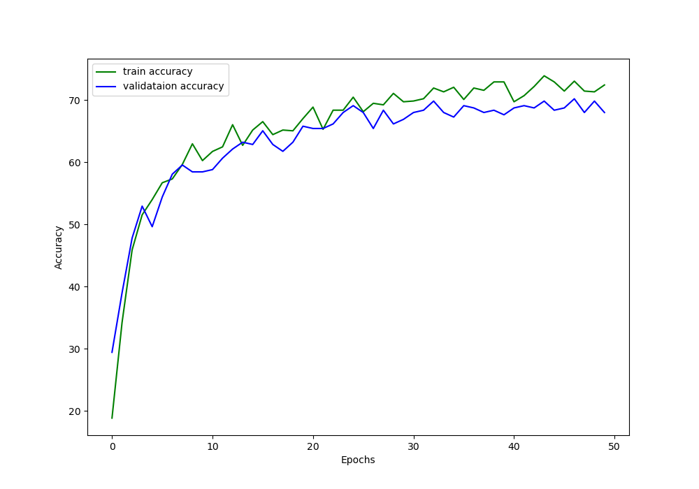
Analyzing the Train Time Augmentation Results

From the console screen outputs, you must have seen that our model is reaching a validation accuracy of 68% by the end of 50 epochs. And the training accuracy is 77.72%. The train loss is also the lowest for both training and validation during the last epochs.

Now, let’s take a look at the loss and accuracy plots that we have saved to the disk. That will give us even better insights.

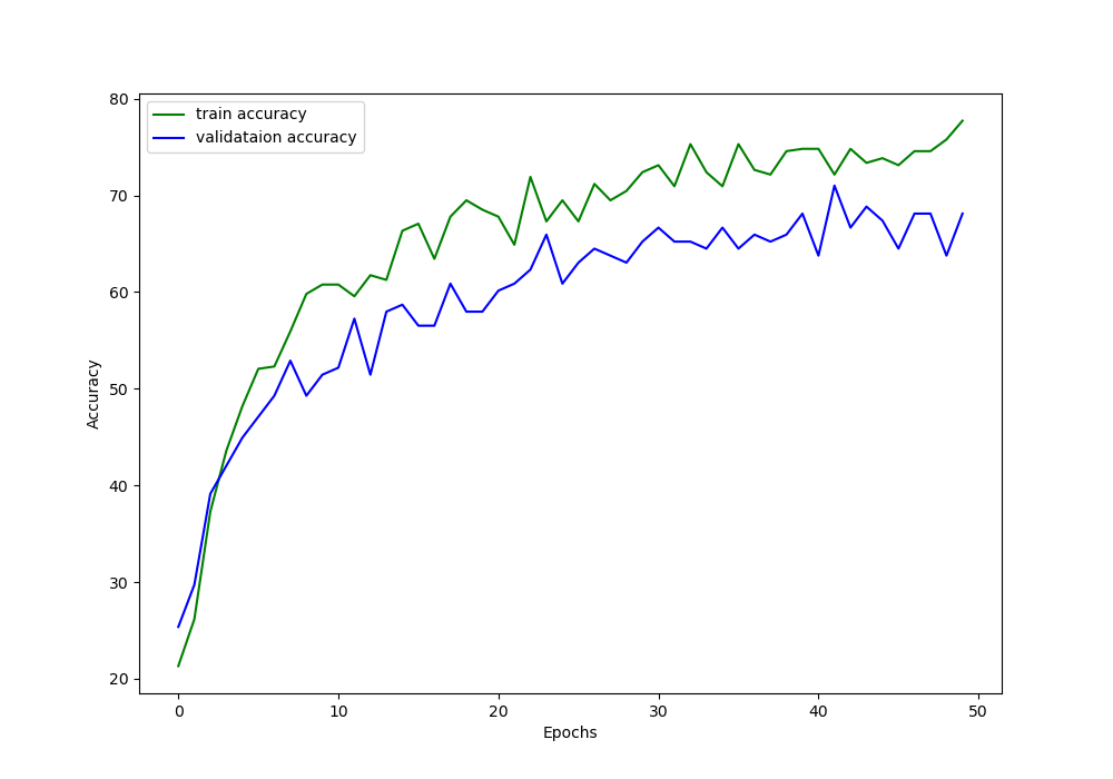
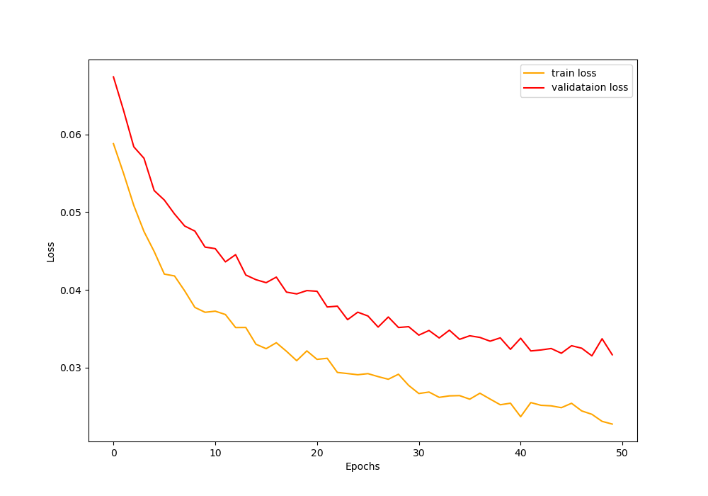
From the above loss and accuracy plots, we can say that the ResNet-18 neural network model is doing just okay after 50 epochs. But there is a clear gap between training and validation values as the training progresses.

The best way to remove this fap is just to get more data. That would make the model train on more data and would also help to validate on more and a variety of images.

Looks like it is a good time to increase the dataset size by applying augmentation to the images and saving them to the disk. We will do just that in the next section.

Expansion of the Chessman Image Dataset using Image Augmentation

In this section, we will write the code for applying image augmentation to the chess images and saving those augmented images to the disk.

As we will apply the augmentation procedure to almost every image in the original dataset, so, we will be able to almost double our dataset size.

All the following code will go into the create_aug_images.py file.

import albumentations
import pandas as pd
import cv2
import os
import numpy as np
import argparse

from imutils import paths
from tqdm import tqdm

parser = argparse.ArgumentParser()
parser.add_argument('-n', '--num', default=50, type=int,
                    help='number of images to augment')
args = vars(parser.parse_args())

We are importing the modules that we require. Starting from line 11, we are defining an argument parser defining the number of images from each category that we want to apply the augmentation on. The default value is 50.

The next block of code define the augmentations that we will apply to the images.

# the augmentations
aug = albumentations.Compose([
                albumentations.Resize(224, 224, always_apply=True),
                albumentations.HorizontalFlip(p=1.0),
                albumentations.ShiftScaleRotate(
                    shift_limit=0.3,
                    scale_limit=0.3,
                    rotate_limit=30,
                    p=1.0
                )
            ])

• So, we are horizontally flipping the images, shifting, scaling, and rotating them as well.
• Note that we are resizing the images into 224×224 dimensions. This is because we are anyway resizing them before training. So, resizing them here should not have any adverse impact.

Remember that we already have a data.csv file containing all the original image paths. We will use that to get all the image paths and then apply the augmentations to the images from each category.

# read image paths from data.csv file
data = pd.read_csv('../input/data.csv')
image_paths = list(paths.list_images('../input/chessman-image-dataset/Chess'))

labels = []
for image_path in image_paths:
    label = image_path.split(os.path.sep)[-2]
    if label not in labels:
        labels.append(label)

print(labels)

for i, label in tqdm(enumerate(labels), total=len(labels)):
    path = '../input/chessman-image-dataset/Chess/'
    images = os.listdir(path+label)
    for i in range(len(images)):
        if images[i].split('.')[-1] != 'gif':
            image = cv2.imread(f"{path+label}/{images[i]}")
            aug_image = aug(image=np.array(image))['image']
            cv2.imwrite((f"{path+label}/aug_{i}.jpg"), aug_image)

• From lines 6 to 9, we are getting all the unique labels (bishop, king, etc.) and appending them to the labels list.
• Starting from line 13, we are going over all the unique categories and getting all the images for that category at line 15.
• From line 16, we start to go over all the images that are in each category.
  • At line 17, we check whether the image has a .gif extension. If so, then we skip that image as applying augmentation to those gives an error.
  • From lines 18 to 20, we read the image using OpenCV, apply the augmentations to the images, and save them to the disk in the particular folder that they belong to.

Now, execute the python file using the following command.

python create_aug_images.py

You should see an output similar to the following.

['Bishop', 'King', 'Knight', 'Pawn', 'Queen', 'Rook']
100%|████████████████████████████████████████████████████████████████████| 6/6 [00:08<00:00,  1.37s/it]

All of the new image will have a file name convention like aug_1.jpg, aug_2.jpg, and so on.

Executing the create_csv.py File Again

Before training on the expanded dataset, we also need an updated data.csv file again. For that we have to execute the create_csv.py file again.

python create_csv.py

This time the output will be this.

100%|████████████████████████████████████████████████████████████| 1085/1085 [00:00<00:00, 1915.30it/s]
   The first one hot encoded labels: [1 0 0 0 0 0]
   Mapping the first one hot encoded label to its category: Bishop
   Total instances: 1106
   Saving the binarized labels as pickled file
                                             image_path  target
   0  ../input/chessman-image-dataset/Chess\Knight\a...     2.0
   1  ../input/chessman-image-dataset/Chess\Queen\00...     4.0
   2  ../input/chessman-image-dataset/Chess\Rook\000...     5.0
   3  ../input/chessman-image-dataset/Chess\Bishop\a...     0.0
   4  ../input/chessman-image-dataset/Chess\Queen\00...     4.0
   5  ../input/chessman-image-dataset/Chess\King\aug...     1.0
...

You can see that we have a total of 1106 images now. This is not exactly double images as we are excluding the .gif images.

Training the ResNet-18 Neural Network Model on the Expanded Dataset

We are all set to train on the expanded dataset. Let’s hope that we get somewhat better results this time with more number of images to train on.

From within the src folder, execute the train.py file in the terminal.

python train.py

The following is the truncated output of the console prints while executing.

Computation device: cuda:0
Training on 829 images
Validationg on 277 images
Loading label binarizer...
Epoch 1 of 50
Training
26it [00:14,  1.81it/s]
Train Loss: 0.0573, Train Acc: 21.11
Validating
9it [00:04,  2.20it/s]
Val Loss: 0.0561, Val Acc: 31.41
Epoch 2 of 50
Training
26it [00:10,  2.41it/s]
Train Loss: 0.0506, Train Acc: 35.22
Validating
9it [00:02,  3.41it/s]
Val Loss: 0.0507, Val Acc: 38.99
...
Epoch 49 of 50
Training
26it [00:10,  2.58it/s]
Train Loss: 0.0237, Train Acc: 75.03
Validating
9it [00:02,  3.27it/s]
Val Loss: 0.0254, Val Acc: 71.84
Epoch 50 of 50
Training
26it [00:09,  2.67it/s]
Train Loss: 0.0230, Train Acc: 76.36
Validating
9it [00:02,  3.19it/s]
Val Loss: 0.0254, Val Acc: 71.12
10.920 minutes
Saving model...

We are training on 829 images and validating on 277 images.

You can see that by the end of 50 epochs, the validation accuracy is 71.12% which is a 3% increment than the previous case.

We can also take a look at the accuracy and loss plots that are saved to the disk.

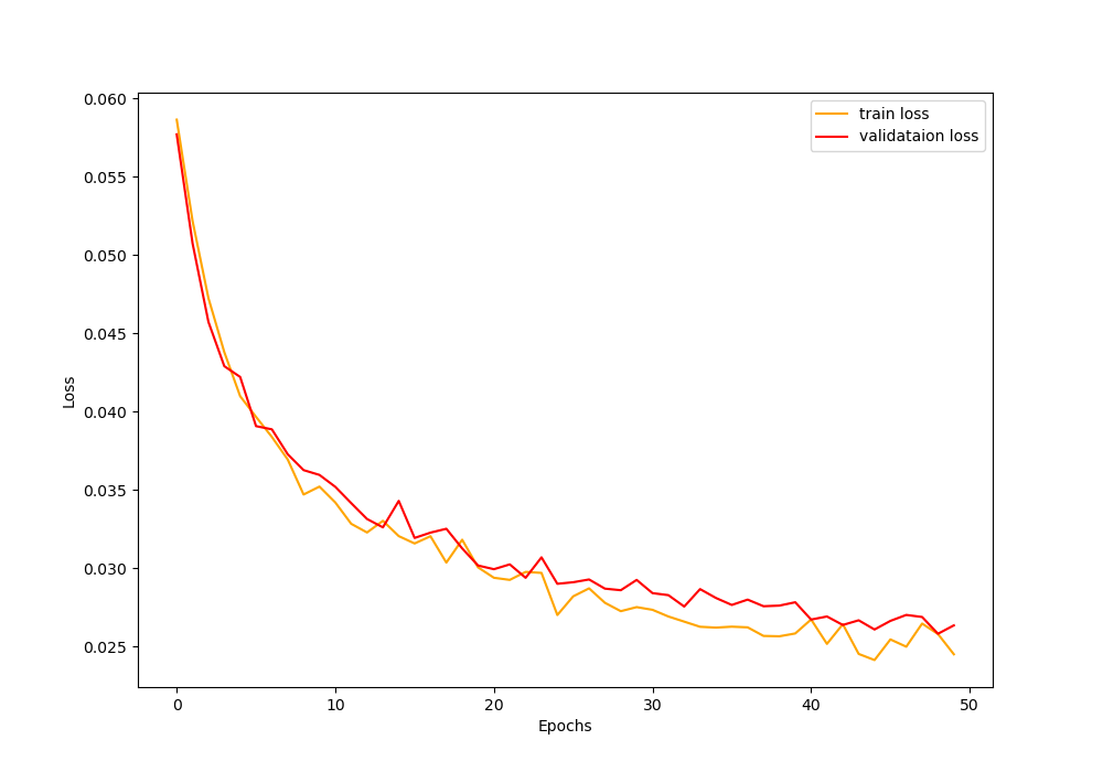
From the above images, we can see that the training and validation accuracy values are following very closely now. This is also true for the training and accuracy loss values.

We are able to reduce the gap between training and validation to some degree by using dataset expansion with image augmentation. We are now very sure that expanding the dataset with image augmentation surely helps.

Moving further, you can also expand the dataset even more with a variety of images.

• You can define two to three types of different augmentation procedures.
• Then you can iterate over the images multiple times and each time apply a different augmentation technique. In this way, you will able to get thousands of images easily for training and validation.
• I hope that you try these steps and tell me about your experience in the comment section.

Summary and Conclusion

In this article, you learned:

• How a small image dataset can reduce the generalization power of a deep neural network model.
• You came to know how to train time augmentation is not always helpful when the dataset is too small.
• You also learned how to carry out dataset expansion using image augmentation and how it helps deep learning and neural network training.

If you have any doubts, suggestions, or thoughts, then you can leave them in the comment section and I will try my best to address them

You can contact me using the Contact section. You can also find me on LinkedIn, and Twitter.